Introduction
What exactly is a quantum computer? In this article, we’ll learn what quantum computing is and how it has amazing potential to let you write software applications in an entirely new way.
See also the research paper, Flying Unicorn: Developing a Game for a Quantum Computer.
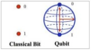
Quantum computing is a technology that uses properties of quantum mechanics to perform calculations at a significantly higher speed and with exponentially more processing capability than classical computers that rely on transistors. While classical computers utilize individual bits that can hold a single state of 0 or 1, quantum computing merges this concept into a single qubit that can hold the value of both 0 and 1 at the same time.
From properties in quantum mechanics, dealing with wave-particle dualities, quantum computers are emerging that can perform computational calculations in an entirely new way, compared to classical algorithms. The potential exists to apply this type of technology to a large range of software products, ranging from database applications, encryption algorithms, search engines, calculations, and even to massively deep-layered neural networks and other branches of artificial intelligence and machine learning.
In this article, we’ll walk through a brief background history of quantum mechanics, just to get an understanding of what makes it so different from classical physics. We’ll then see how this applies to computers, culminating in the concept of quantum computing. Finally, we’ll learn how to create our own software programs that run on real quantum computers. We’ll start with your very first “Hello World” in quantum programming, and then move on to examples that demonstrate some of the unique properties of quantum mechanics, including superposition and entanglement, ending with our very own quantum game, Fly Unicorn.
Classical Physics and Quantum Physics
Before quantum physics was discovered, the world was quite comfortable with classical physics. Classical physics does a good job at explaining the macroscopic world. That is, the world that we can see and feel all around us, containing massive particles, is explained and described by classical physics. However, as you move smaller into the microscopic world, things begin to behave quite differently. When quantum physics emerged, there were several distinctly different concepts that made it unique from classical physics.
When Things Get Very Tiny
In the macroscopic world, we’re used to seeing and experiencing things around us that we can see, hear, feel, and touch. For example, you can pick-up an apple and toss it on the ground. You know that the apple will hit the floor and stop. It certainly won’t fall through the floor and continue to the center of the Earth. Likewise, when you sit on a chair, you know that the chair will hold your weight. You won’t simply fall through the chair to the floor. This is due to electrostatic force between atoms within the chair and your body. When the atoms of the chair come close enough to your body, the charges of their electrons and your own repel each other, thus causing the chair to hold your weight.
In the world that we can see, these properties make sense. However, in the microscopic world where quantum physics takes effect, these properties can be quite different. Let’s briefly take a look at the three key concepts that make quantum physics so unique.
Intrinsic Granularity
When you ride on a swing hanging from a tree, you sway forward to back with graceful ease. You feel the smooth movement of the swing moving up and down. If you stop swaying your legs, you’ll feel the swing gradually beginning to slow down, reaching a slightly lower height each time it swings up, until it eventually comes to a stop. What you don’t feel, however, are discrete bursts of force against the swing, repeatedly causing it to slow down at each interval of energy. If you were tiny enough, the swing were small enough, and the length of the rope was miniaturized to a microscopic level, you would actually begin to feel individual bursts of slowing down against the swing until it comes to a rest.
In quantum physics, this is the concept of pixelation. In the microscopic world, physical quantities no longer move smoothly from one state to another, rather they become pixelated. On a larger scale, something that appears to have smooth flowing movement (such as a child on a swing), actually has discrete bursts of energy, thus individual bursts of movement, at the microscopic scale.
While a child on the swing is unable to sense these discrete chunks of movement as the swing comes to a stop (because these bursts of energy are so tiny), they would become apparent at the microscopic level.
Logical Inconsistencies
The quantum world also differs from classical physics by its effect of logical inconsistencies from what we’re used to experiencing. In the quantum world, it’s possible for an object to appear simultaneously in multiple places. This is due to the effects of probability at the microscopic level, which permits an electron or photon to be present in multiple locations at the same time.
Further, quantum objects can even suddenly appear out of nowhere, spontaneously popping into existence from absolutely nothing. It’s even theorized that this occurs on a regular basis in our universe. However, the reason that you don’t suddenly see a pumpkin materialize on your doorstep is due to the fact that as the particle becomes larger in scale, the duration of time that the spontaneously appearing particle can exist becomes increasingly shorter. In the microscopic world, particles are theorized to be able to pop into existence for an extremely brief amount of time. As these particles increase in size, the time duration that they can exist decreases. A particle the size of a tiny speck of dust could materialize into existence, but it would only exist for such an unimaginably short amount of time that it would likely never be detected or realized. These types of unthinkable properties of quantum physics are just some of the factors that make it so unique from classical physics.
Inherent Uncertainty
The third unique difference of quantum physics from classical physics is the pure amount of uncertainty that must be taken into account when dealing with the microscopic world.
In classical physics, measurements are traditionally certain and clearly understood with a precise degree of accuracy. However, in quantum physics, results are based upon probabilities with a degree of error. You can never be completely sure of the precise and exact location and speed of an electron moving through space. This is due to Heisenberg’s Uncertainty principle. We can obtain a closer precision of a particle’s position if we sacrifice accuracy for its velocity, but you can’t have both.
This uncertainty in the quantum world is due to the fact of simply measuring a particle’s position.
To measure a particle, such as an electron, we require light. Light is in the form of photons. We need this in order to observe a particle, otherwise we simply can’t see it in any manner. Since observing a particle requires at least a single photon to hit it, and that photon must interact with the particle, it will result in transferring its energy to the particle. This results in the particle’s position and/or speed changing, due to the impact by the photon and transference of its energy to the particle. In this manner, the simple act of observing an object at the microscopic level changes its position and velocity accordingly. Therefore, we can never know exactly where or how fast an object is moving in the quantum world, because the moment that we observe it, it’s changed!
To make matters worse, if we try to achieve more precision in our measurement, more photons are required. However, this results in more bombardement on the particle, thus shifting its position and velocity even further. If we use less photons to try to minimize any movement effect, less energy will be transferred to the particle, but our ability to detect its position with precision will be compromised and made more difficult. In both cases, our accuracy for detecting the particle’s position and speed are subjected to uncertainty.
With this basic comparison of classical physics to quantum physics, let’s take a look at how quantum physics is applied to computing. We’ll start with the famous double-slit experiment.
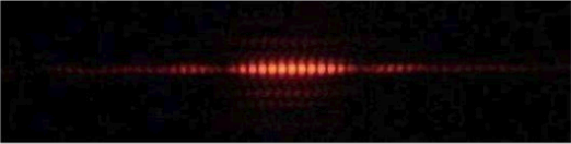
The Double-Slit Experiment
The double-slit experiment demonstrates the unique property of wave-particle duality that exists in the quantum world. This is key behavior that leads to the properties of quantum computing. Let’s take a look at the experiment and its results to understand how quantum mechanics, specifically the behavior of electrons, occurs in the microscopic world.
Tennis Balls
To start off, imagine a wall with two slits in it. Imagine throwing tennis balls at the wall. Some will bounce off the wall, but some will travel through the slits. If you mark all the spots where a ball has hit the second wall, you’ll see two strips of marks roughly equal to the same shape as the slits that they’ve passed through.
This is pretty easy to imagine, since the tennis balls that make it through the slits hit the walls at the same general location from the holes. You could use the same concept as an hourglass pouring sand through its slot. The sand begins to form a pile directly under the hole at the top of the hourglass. Likewise, the tennis balls being fired at the wall, travel through the slots in the wall and form two impact zones against the wall behind it.
This is the idea to how particles behave at the macroscopic scale.
Light
Now imagine shining a light at a wall with two slits. As the wave of light passes through both slits, it essentially splits into two new waves, each spreading out from one of the slits. These two waves then interfere with each other, causing a stripe pattern, called an interference pattern. In contrast to particles which only formed two strips, with photons we get three (and more) strips due to the interference pattern from the waves.
This is the same effect as waves in the ocean striking each other, cancelling out and building larger waves in the process.
Next, let’s take a look at the quantum world.
Electrons
Imagine firing electrons at our wall with the two slits, but assume that we close one of the slits for the moment. So, we have a single slit in a wall and we begin firing electrons at the wall.
Many of the electrons will hit the wall and simply be blocked. However, some of the electrons will pass through the open slit and strike the second wall behind it, just as the tennis balls did. Each spot where the electrons impact the second wall will form a strip roughly the same shape as the slit. So, the electrons are behaving just like tennis balls (i.e., particles).
Now, consider what happens if we open the second slit and fire the electrons at the wall.
You might expect to see two rectangular strips on the second wall, similar to the tennis balls, being formed from the electrons passing through each of the two slits and impacting the wall behind. However, the actual result is surprisingly different!
As it turns out, the spots where electrons hit the second wall, build up to replicate the interference pattern from a wave. So, electrons are behaving as a wave, just like the photons!
Thinking that maybe the electrons are interfering and bouncing off of each other, in mid-flight, to create the interference pattern, we can try firing the electrons one at a time. This way, there is no chance for them to interfere with one another. However, this time, the interference pattern still remains! Even stranger, each individual electron contributes one dot to the overall interference pattern on the wall.
Let’s take this one step further.
Thinking that the electron might be somehow splitting and passing through both slits (afterall, we’re only firing one electron at a time), you could place a detector in front of each slit to see which one it goes through. This is where we can start to see the extraordinary results of quantum physics. After placing a detector to observe the electrons, the impact pattern on the second wall turns into the particle pattern of two solid strips, as seen in the original experiment with particles! That is, the interference pattern disappears. Somehow, the very act of looking causes the electrons to travel like the tennis balls. Even more odd, this same result occurs whether the detectors are placed in front or in back of the open slits.
It’s almost as if the electrons know that you’re looking at them and decide to behave like particles and the moment that you stop peeking, they go back to behaving like a wave.
The double-slit experiment demonstrates that objects at the microscopic level, such as electrons, combine characteristics of both particles and waves. This is the concept of the famous wave-particle duality of quantum mechanics. The wave-particle duality describes that the simple act of observing or measuring a particle in a quantum system has a distinct effect on the system itself. Further, since the act of observing a quantum system causes its behavior to change, this explains the idea behind the measurement problem of quantum mechanics.
What is Quantum Computing
There are several key differences between classical computers that we use today, when compared to quantum computers. These factors include the amount of data that can be processed within a single compute-cycle, as well as the speed of processing information.
Classical Computing
The computers that we use today rely on transistors. A transistor is a miniature switch, that allows electricity to flow between wires. When the transistor has a “high” voltage measurement, the resulting bit value can be deemed to be 1. Likewise, when the transistor has a “low” voltage measurement, the bit value is considered to be 0. There are millions of these tiny transistors within a typical CPU chip. For example, the Intel Core i7 CPU has 731,000,000 transistors.
Naturally, since electricity is flowing across wires and through gates, it’s limited by the speed with which it can move across the wires. Additionally, the transistor is only capable of representing a single value of off or on, 0 or 1 respectively. Each transistor can represent this value at a single time - that is, a single transistor can be low or high, open or closed, 0 or 1, but never both at the same time.
As a classical computer can represent a single bit of information with a value of 0 or 1, the operation is XOR. That is, the value of a bit can only be 0 or 1, but never both simultaneously. Therefore, a classical computer can process n-bits in a single CPU cycle.
The representation of a bit as 0 or 1 on a classical computer may seem somewhat obvious and hardly a limitation. However, when we compare this to what a quantum computer can offer, we can begin to see a remarkable quantum advantage.
Quantum Computing
Quantum computing relies on a completely different technology for representing bit information, compared to classical computers. Quantum computing takes advantage of the properties of quantum physics in order to perform calculations. On a quantum computer, transistors are no longer required. Instead, electrons or photons are measured according to their quantum properties, such as spin, resulting in a calculation of 0, 1, or a probability between. Because of the unique properties of these particles at the microscopic level, they can hold the value of 0 and 1 simultaneously until measured. This property in quantum mechanics is called superposition.
Representing a single bit (also called a qubit) of information as both 0 and 1 at the same time is a significantly different property from classical computing. Consider what this means for processing power on a quantum computer.
A single qubit can hold a value of 0 and 1. Therefore, a quantum computer with 1 qubit can hold 2 bits of information (0 and 1). Likewise, a quantum computer with 2 qubits can hold 4 bits of information (00, 01, 10, 11). Going a bit further, we can see that 3 qubits gives us 8 states, 4 gives us 16, 5 gives us 32, and so on. In this manner, a quantum computer can process 2^n bits of information simultaneously per compute cycle.
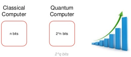
This represents an exponential difference in processing power compared to classical computing that relies on transistor technology. If we extrapolate on the number of qubits, a 50-qubit quantum computer can process 2^50 bits of information in a single cycle, or 1e+15 bits of information, compared to a classical computer which could simply process 50 bits of information with the same number of transistors.
The difference between classical and quantum computing becomes very apparent when we see the exponentially larger amount of information that can be processed in a single cycle on a quantum computer, compared to its classical counterpart.
Let’s see what this actually means for processing data.
500 Petabytes of Facebook Data
One of the prime targets for quantum computation is big data. Now, big data is huge! And, it’s only going to get bigger. Let’s consider an example of big data at Facebook.
Big data can be calculated in petabytes. This is because it’s so large. One petabyte is equal to 10^15 bytes. Since we want to compare this to qubits, which are described by 2^q states, instead of 10^15, let’s say 2^50 bytes, since these values are similar. This means that a quantum computer with just 50-qubits can process a petabyte of information in a single calculation cycle!
If Facebook stores data for 2 billion accounts, this could be in the magnitude of 500 petabytes in the near future. A quantum computer with 60 qubits can perform a calculation on this much information within a single cycle.
Cracking RSA
Another natural application of quantum computing is code breaking. This is due to the massively parallel processing that qubits can offer, compared to their classical counterparts. While a classical bit can only represent a single 0 or 1 value at a time, quantum qubits can represent both, while in superposition, simultaneously. In this manner, cracking an RSA key, which consists of identifying two prime factors, could be an easy task for a quantum computer.
A quantum computer capable of breaking RSA 2048 would require about 4,096 qubits.
How Does a Quantum Computer Work
Now that we can see the exponentially more powerful processing power with quantum computing, how exactly do we build a quantum computer?
Quantum computing relies on quantum mechanics. This means that we’re manipulating particles at the microscopic scale. Some companies, including IBM, Google, and Intel, have already built machines for accessing quantum computational functionality.
For example, IBM Q uses superconducting loops where electricity can flow without loss. An electric current oscillates back and forth within the loop, upon which microwaves can be used to excite the state of the electrons (i.e., qubits) to perform operations. In order to stabilize the electrons and isolate them from outside interference, an extremely cold environment, at 0.015 Kelvin (near absolute zero), is required.
Other methods for creating a quantum computer include ion traps, used by IonQ, as well as silicon dots, used by Intel.
In addition to building a quantum machine, we need a way of interacting with the qubits and translating them into a medium that can be used with classical computers that we use every day.
We can do this by using a classical computer process for receiving the input. This input is then passed to the quantum computer, which then processes the information, for example, using a quantum computational algorithm. The result from the computation is then passed to a classical computer which interprets the results and outputs to the user.
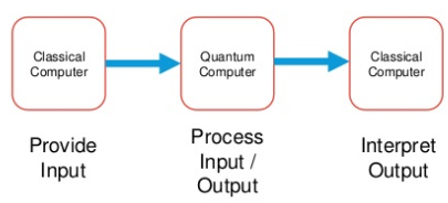
In this manner, a quantum computer sits between two classical computer processes - one for input of data and one to render the output.
Transitioning From Classical Computing to Quantum Computing
Now that we’ve connected the theory behind quantum mechanics with the world of computing, we can see how quantum physics relates to a computing medium that we can actually use to perform calculations and process information.
Since quantum computers rely on quantum physics, they contain very unique and distinct properties from classical computers that we’re used to. As we’ve discussed, the process of superposition of an electron allows us to represent a bit as a probability of holding a value of both 0 and 1 at the same time. Additionally, we have the concept of entanglement between qubits, which brings us further possibilities for changing the way that we write software. We’ll discuss entanglement in just a bit. However, first let’s take a look at a quantum computing algorithm to see how it’s different from a traditional transistor-based computing algorithm and the kinds of advantages that quantum computing can give us.
The Deutsch-Jozsa Algorithm
The Deutsch–Jozsa algorithm is a quantum algorithm created to demonstrate the difference between classical and quantum computer calculations. The algorithm itself is not particularly practical for a specific purpose, although it provides an easily understandable way of seeing how a quantum algorithm significantly differs from a traditional computing one. Additionally, it allows us to see the exponentially increased performance of a quantum computer compared to a classical one, in both memory and speed.
In the Deutsch-Jozsa problem, we are given a black box quantum computer known as an oracle that implements a function. The function takes n-digit binary values as input and produces either a 0 or a 1 as output for each value.
The oracle function is guaranteed to always be either constant (0 on all outputs or 1 on all outputs) or balanced (returns 1 for half of the input domain and 0 for the other half). The goal of your algorithm is to determine if the function is constant or balanced.
Traversing the Array
Now, upon first glance, a naive approach might be to simply iterate across your array of input values and call the oracle function for each bit in your array. You can look at the output from the oracle (0 or 1) and if you see all 0’s or all 1’s upon completing the array iteration, then you know the oracle is constant. Likewise, if you see a mix of 0’s and 1’s then you know the oracle is balanced.
Of course, you might realize that you don’t actually have to traverse the entire input array. We can optimize our algorithm by checking against just over half the input. That is, we send the first combination of n-bits to the oracle function and check its output. Let’s assume we get a 0. We send the second input combination and get back another 0. So far, it’s looking like a constant function. If we read a different output (1) for any other input at this point, then we now know that we’ve read both 0’s and 1’s for the output, thus the oracle function must be balanced. If we continue to read all the same values up to the midpoint of combinations for the n-bits (in this case, we’ve read all 0’s), we can read the result for the (2^n / 2) + 1 combination and check if its output is 0 or 1. If it’s different (1) then we know the oracle is balanced and we can stop traversing. Likewise, if the result is the same (0) then we know the rest will be the same as well, and the oracle function is constant.
Getting Our Hands Dirty
Let’s see what the Deutsch-Jozsa Algorithm looks like with a quick example.
Consider we have a 5-bit input to check if the oracle is constant or balanced. That is, for every combination of 1’s and 0’s over 5-bits, the oracle will either always return the same value (constant) or equally 0 and 1 for exactly half the results (balanced).
For a 5-bit array there are 2^5 combinations, or 32 combinations to check against the oracle. We know that we can determine if the oracle is constant or balanced with a classic algorithm by checking against the oracle for (2^n / 2) + 1 attempts, or 17 tries (just over half the number of combinations). If the oracle returns a different value for any of those combinations, we know that it’s balanced. If they’re all the same, we know that it’s constant.
An Almost Best-Case Scenario
Consider the following input and resulting oracle response, where we only need to call the oracle 6 times before determining that it’s balanced.
1 | 1 00000 => sent to oracle => 0 |
The above set called the oracle 6 times before receiving a differing value. Thus, we immediately know that the oracle is balanced and no further checks are required.
A Worst-Case Scenario
Let’s consider an alternative scenario. In this case, the oracle returns the same value all the way up to half-way through the number of combinations.
1 | 1 00000 => sent to oracle => 0 |
In the above scenario, we’ve called the oracle for every combination of the n-bit array up to half-way through the number of combinations and have received back a constant value of 0 each time. Since we’re half-way through, we know that if we read the next value (the 17th combination) and receive a differing result from the oracle, that the oracle is balanced (and, in fact, that it will return 1’s for the remainder of combinations). Likewise, if it returns the same value for the 17th combination, we know that the oracle is constant. In both cases, there is no need to call the oracle for the other combinations.
Just a Single Call with a Quantum Computer
On a classical computer, the best case occurs where the function is balanced and the first two output values that happen to be selected are different. Since we’ve just read two different values, we know the function must be balanced. Remember, the function is guaranteed to be either balanced or constant and will always return either all the same value for every input or a combination of values, but equally balanced counts of both 0 and 1.
To prove that the function is constant, we had to evaluate just over half the set of inputs, checking if their respective outputs are identical.
For a conventional deterministic algorithm where the input array contains n bits, we can solve this problem with (2^n / 2) + 1 (or 2^(n-1) + 1) evaluations in the worst case scenario.
With quantum computing, the algorithm can solve the problem with just a single function evaluation! We only have to call the oracle function one time. This is exponentially faster than any possible deterministic classical algorithm.
The Deutsch-Jozsa algorithm is a straight-forward way to demonstrate the capabilities of quantum computing and how differently the algorithms can behave. It will become important to keep this in mind as you transition to quantum programming, in order to create new algorithms that can work with quantum technology.
The Concept of Quantum Entanglement
So far, we’ve seen how quantum computing works by utilizing properties of quantum physics. We’ve discussed superposition, allowing a qubit to simultaneously hold the value of 0 and 1 at the same time, until measured.
Quantum mechanics can be even more mysterious than we’ve already seen. In addition to the behavior of electrons as both waves and particles, there is also the concept of quantum entanglement. This is another feature of quantum physics that can be leveraged in computing to create new algorithms that can perform in ways unavailable to classical computers.
So far, we’ve been talking about qubits, which store information of 0 and 1. Qubits can actually interact with other qubits in their respective states. When they do this, it is called an entanglement.
A qubit can not actually be measured without measuring all entangled qubits. Additionally, this entanglement of qubits can occur over great distances of separation. One qubit can influence another qubit that is physically far away. The current record held for entangling two qubits (as of 2018) was performed via satellite, with a distance record of 748 miles. Imagine being able to harness this feature across vast distances of space.
Einstein called the process of quantum entanglement as “spooky action at a distance”. This is because the two electrons can be far away from each other, and if one is modified or measured, the other electron will hold the same value. How exactly this works, is still under debate and exploration by quantum physicists. However, there are several prevailing theories on how these particles maintain entanglement.
Collapse of the Wave Function
Within a quantum system, whether it be an electron, photon, microscopic particle, a wave function can describe the behavior, movement, and velocity of the particle. In this manner, quantum physics allows us to describe a quantum particle and even predict the future movement and velocity accordingly. This can be expanded to larger systems, each being described by a specific wave function.
As long as a particle is in the superposition state, its wave function exists and is valid. However, upon measuring the value of the particle, this single action causes an immediate collapse of the wave function. This results in the particle holding the value of 0 or 1 (no longer both simultaneously) and the wave function is collapsed.
It’s not exactly understood how the wave function is able to collapse instantaneously, without any delay whatsoever. However, this is part of ongoing research. When a wave function does collapse and the particle is no longer in superposition, there is still the question of how do two entangled quantum particles communicate with each other to synchronize the measured value accordingly? Recall, when one entangled electron is measured, the other electron will hold a corresponding value regardless of distance.
Multiple Universes
One theory behind how entanglement occurs is through the multiple universe theory. This theory explains that multiple universes exist. The moment a particle in superposition is measured, its wave function collapses instantaneously, resulting in a value of 0 or 1. However, since a quantum particle’s value is a probability of 0 and 1, the multiple universe theory states that one universe exists with the electron in a measured value of 0, while a second universe is branched out and created instantaneously with a measured value of 1. In this scenario, both universes are exactly the same with the exception of the single electron’s measured value.
Imagine a researcher using a measurement tool on an electron to check its value. The moment the measurement is made, a clone universe is created. In both universes the researcher exists. In both universes the measurement tool exists. The only difference between the two universes is that in one, the researcher reads a value of 0 from the electron. In the second universe, the research reads a value of 1. In this manner, the superposition still upholds its quantum property of allowing the electron to hold a value of 0 and 1.
Now, a single electron changing its value in the universe might not sound like a big deal, but imagine the repercussions of electron after electron changing its values across millions and billions of years in the designated universe. Imagine how many measurements are made on a quantum system over this amount of time. A measurement doesn’t have to exclusively be a piece of digital equipment in a research lab. It can be the simple act of looking at a particle (as this results in photos hitting the particle, thus collapsing the wave function) or even possibly non-conscious measurements such as impacts with other objects and entities.
In the multiple universe theory, there would exist an infinite number of universes since the beginning of time, with even more being created at every instance of time. These universes are perpendicular to each other, which would prevent the possibility of ever being able to communicate with one another. However, some theorists believe it may be possible to communicate with two branched universes shortly after their creation.
An Invisible Force
Another theory behind how entanglement in quantum mechanics exists is through the idea of an invisible flowing force. Imagine the creation of two electrons that subsequently become entangled. The electrons are then flug far out into space away from each other. The invisible force theory describes a hidden connecting wave between the two electrons the spans the entire distance between the electrons, connecting them across vast distances of space. When one electron is measured and its corresponding wave function collapses, this indivisible force somehow transmits that measurement information to the entangled electron, thus passing the value across.
Since the invisible force theory describes quantum systems being connected through a hidden wave, it reasons that every single particle and atom in the entire universe could be connected to one another through a hidden force.
The repercussions for both of these entanglement theories are certainly impressive to consider.
No Free Will
A third theory of entanglement describes the idea of two entangled quantum particles already having their values determined at the time of their creation. In this manner, when the two particles travel vast distances away from each other and are subsequently measured, they will already hold the expected corresponding value without ever actually changing or being affected by those changes while in transit from creation. If this were true, it would mean that every particle, including massive ones, and even potentially all humanity, would be predestined to certain fates that have already been determined upon the creation of the universe.
Communication Faster Than the Speed of Light, Not So Fast
Given the concept of quantum entanglement and how it can occur over great distances, seemingly instantaneously, one might wonder if it would be possible to communicate faster than the speed of light.
With quantum entanglement, information is not actually being sent faster than the speed of light. While two entangled qubits will indeed share correlated values (if qubit A is 1 then qubit B is 1 as well) even over vast distances, it is not possible to force the state of qubit A to a specific value in an attempt to reflect that value to qubit B. The moment you perform this operation and subsequent measurement on qubit A, the entanglement is broken. At this point, qubit B will now measure as a random value.
Quantum Encryption Key Distribution
To dig a bit deeper into quantum entanglement and its relationship to communication speed, let’s look at the idea of quantum encryption key distribution. Quantum key distribution is the concept of two parties securely generating an encryption key through the usage of quantum mechanics.
Consider a rover being sent to Mars. Let’s suppose we need an encryption key in order to communicate with the rover, but we don’t want to create this key and hardcode it into the rover before-hand for fear of it being compromised. Let’s also suppose the encryption key will consist of just two bits. Of course, this is not a particularly strong key, but it will suffice for this example.
To create the encryption key, four qubits are created. Two are placed into superposition and subsequently entangled to the other two. The two qubits in superposition are held on Earth. The other two qubits are sent with the rover to Mars. Once the rover arrives on Mars it needs to determine an encryption key. Of course, Earth also needs to know this encryption key in order to read the messages that the rover transmits. To do this, we measure the two qubits on Earth that are in superposition (remember, they could result in any of 4 values [00, 01, 10, 11]). The moment we measure these two qubits, the rover’s two qubits will hold the same values, due to entanglement.
Let’s suppose on Earth that the measurement results in the value 01. When the rover measures its qubits, it will also see the value 01. We now have an encryption key and can begin sending messages, via a classical communication channel, between Earth and Mars.
If an eavesdropper somehow intercepted either of the parties qubits and measured them to see the key, this would break the entanglement. When the other party then measures their own qubits, they would measure completely random values. Thus, any attempt to communicate using this key would fail, since both parties would now have different random keys. They could now choose to re-generate a key by creating a new set of entangled qubits.
With quantum key distribution, it may seem as if the key’s value traveled faster than the speed of light (the instant the qubits were measured upon Earth, the rover’s qubits matched them accordingly). However, this actually required sending the two qubits via classical means on the rover’s spacecraft and measuring them at a later time. Additionally, the qubits could not be coerced to a specific value. The random values that the first two qubits measured would be likewise present in the second pair.
There are certainly some very interesting philosophical concepts surrounding quantum physics to be taken under consideration. However, let’s stick with the science that we can use today, specifically with quantum computing.
Writing Your First Quantum Program
Now that we’ve covered a very high-level overview of quantum physics and its relationship to quantum computing, let’s take a look at how we can start writing software on a quantum computer!
We’re going to be using the QisKit framework for utilizing the quantum machine located in IBM’s facility. QisKit is an open-source framework for quantum programming and contains both a simulator for executing quantum programs and also an API call to send the request to an actual quantum computer at IBM labs and send back the result.
Installing QisKit and IBM Q
Before we can started with the code, we’ll need to install a quantum programming framework.
We’re going to be using the QisKit library, so you’ll need to install QisKit on your computer. You can do this by using pip with Python3.
Once you have the library installed, you’ll also probably want to create an account with IBM Quantum so that you can run quantum programs on an actual quantum computer (instead of just the simulator).
After creating an account with IBM Quantum, go to the “My Account” page, and locate the field to create an API key. Copy this key, as you’ll be using it in the code examples that follow.
Hello World
Let’s start with the most basic, “Hello World”, of quantum computing. We can begin writing our first quantum program, as shown below.
1 | import qiskit |
Upon running the program, you should see the following output.
1 | Hello World! {'0': 100} |
In the above program, we’ve first imported the required libraries for accessing the QisKit API. Next, we set our API key in order to use the quantum computer at IBM Q. Our real code starts where we initialize our first qubit.
We begin by making a call to QuantumRegister(1) which obtains a single qubit for us to work with. We also create a classical register, in order to interpret the result of a qubit into a form that a classical computer can understand. Finally, we tie the two together with a QuantumCircuit command, which is effectively our program.
Now that we have a qubit prepared, we can measure it and obtain its value. When we finally run the quantum program, we obtain the result, which should appear similar to {‘0': 100}. This means that the quantum computer has run the calculation for our program and obtained the value of 0 100 times. Because quantum programs are still susceptible to a degree of error (sometimes averaging an error rate of 10%), you may want to perform the calculation multiple times. In this case, we’re running it 100 times. You can specify the number of times to run the quantum program with the shots parameter in the call to qiskit.execute().
Now, since all we’re doing in our quantum program is measuring a qubit in its ground state and nothing more, our qubit should always have the value 0. And so, we see that for all 100 attempts, we indeed get back a result from the simulator of 0.
In addition to running the quantum program on the simulator, we can also run it on a physical quantum computer at IBM Q. To do this, add the following code to the end of your program.
1 | # Execute the program on a real quantum computer. |
The above code is almost the exact same as we used for the simulator, with the only difference being the type of backend that we send our code to run on. In this case, we’re using an IBM Q backend machine and obtaining the results.
Notice that due to the error rate on the physical quantum computer, our counts are a little different. We see an output similar to the following.
1 | Hello World! {'0': 98, ‘1': 2} |
In the case of running on a real quantum machine, we expect our qubit to measure a value of 0. When we run the program 100 times, we see that most of the time we get back a value of 0 as expected. However, 2 of the attempts return a value of 1. This is simply to be expected when working with the volatility of quantum computers.
Using Superposition, Entanglement, and Bell States
For this next example, we’re going to use the property of superposition and entanglement to create a Bell State between two qubits. In this manner, we will connect the value of one electron to the value of another.
First, let’s create a helper method for running the quantum program on the simulator versus a real quantum computer. This code is shown below.
1 | import qiskit |
The first thing that we’ve done is to define a method run(). This methods lets us specify which environment to run the quantum program on (sim for simulator, and real for a physical quantum computer). This will help simplify our quantum programming code.
Measuring Two Qubits in Their Initial States
We’ll start with a simple program to measure to qubits in their initial states. This is almost exactly the same as our Hello World program, except that we’re measuring two qubits instead of just a single one.
1 | # |
The above program should give you the output shown below.
1 | {'00': 1024} |
As expected, both qubits should measure a value of 0.
Creating a Bell State
Next, we’re going to use two qubits to create an entanglement and represent a bell state.
1 | # |
In the above code, we begin by creating two qubits and two classical registers to hold their final values. Next, we execute the method h() on the first qubit to place it into superposition. This command executes a Hadamard gate_gate) on the qubit, placing it into superposition so that it has an equal probability of holding the value 0 or 1.
Next, we entangle the first qubit with the second by using a controlled-not gate, with the cx() method. This entangles the two qubits so that their values will correspond to each other. Specifically, the controlled-not gate inverts the value of the second qubit when the first qubit is 1. That is, when the first qubit holds a value of 0, the second qubit will remain unaffected. However. when the first qubit holds a value of 1, the second qubit will be inverted (from 0 to 1, or 1 to 0). This occurs within superposition and is thus part of the entangled states between the two qubits.
When we finally measure the resulting qubit values, we will expect to see an equal distribution of 00 and 11 from the resulting measurements. Since the first qubit is in superposition, and since the second qubit is entangled with the first (and since we perform no other operation on either qubit), any value that the first qubit holds will be reflected in the second qubit through quantum entanglement.
When we run the program, we see the following output.
1 | {'11': 494, '00': 530} |
In the above output, about 50% of the time we see 11. Likewise, about 50% of the time we see 00. Notice that in both cases if the first qubit held a value of 0 so did the second qubit. Likewise, for the value of 1. In no case do we see a split of 01 or 10. This is because the controlled-not operation entangles our two qubits, ensuring their values remain connected.
Superdense Coding for Alice and Bob
Let’s now see an example for superdense coding with a quantum computer. With superdense coding you can send two classical bits of information by only manipulating a single qubit.
The motivation behind superdense coding is that suppose there are two individuals, Alice and Bob. Alice owns a qubit. Bob owns a qubit. Alice wants to send the value 01 to Bob by only sending him her own single qubit. In order to do this, Alice and Bob’s qubits must already be entangled. Alice can then modify her own qubit (which is in superposition) accordingly, and then send the qubit to Bob. When Bob measures the two qubits, he’ll see the desired value from Alice of 01. Thus, two bits of information were transmitted by only modifying a single qubit.
This can be performed through a series of steps. First, we’ll create two qubits. We’ll place the first qubit into superposition. Next, we’ll entangle the two qubits. We can now hand Alice the first qubit qr[0] and give Bob the second qubit qr[1].
Alice and Bob both fly off to far away places.
Now, in order to setup the correct value to transmit to Bob (when he measures the qubits), Alice can manipulate her qubit. She can leave her qubit as-is, to represent the value 00 to Bob. She can apply an invert operator program.x() on her qubit to represent the value 01 to Bob. She can apply the program.z() operator to represent the value 10 to Bob. Finally, she can apply both the program.x() and program.z() operators to represent 11 to Bob.
1 | # |
Upon running the above code, you should see the following output after Bob measures the two qubits.
1 | {'01': 553, '10': 471} |
In the above output, remember that our first qubit is in superposition, holding the values 0 and 1 simultaneously. When we run our program to send Bob the value 01, we can see in our output that 50% of the time we will see 01 and the other 50% of the time we will see 10, as expected.
Writing a Quantum Computer Game: Fly Unicorn
Let’s build something fun as a final example with quantum computing. We’ll create a game about a flying unicorn!
One of the unique properties of quantum physics is the uncertainty principle, which states that you can’t know the exact location or velocity of a quantum particle, such as an electron, when measuring it. The simple act of measuring, itself, affects the position and velocity of the electron by bombarding it with photon(s). Due to this, there is inherent uncertainty in quantum measurements.
Quantum uncertainty manifests itself in computing in the form of an error rate when measuring calculations for expected values. In addition to inherent uncertainty, the error rate is further exacerbated by the technology for creating quantum particles itself. For example, in our projects we’re using IBM Q and their technology for generating qubits, which relies on a supercooling technique. When the electrons are cooled low enough it helps to decrease the error rate upon performing operations and taking measurements. However, an error rate still exists.
We can utilize the inherent quantum error as a sort of random number generator for our game. Let’s see how it works.
Fly Unicorn
We’ll start with the best part of the game, the actual output. Below is an example of the game running.
1 | =============== |
In the game, the player is flying a unicorn with the goal being to reach the castle in the clouds. The player can choose to fly up or down at each round. When the player chooses to fly, we need to determine how much altitude the unicorn gains or loses. Now, if we simply add/subtract a constant value of 100 at each round, the game could certainly be played, but it wouldn’t be very interesting.
Instead, at each round, we calculate a random value corresponding to how close the unicorn should be from the goal, and use the error rate returned from the measurements of the qubit to determine the resulting altitude gained or lost.
In effect, we’re using quantum physics, with an electron to be specific, as a qubit and turning it into a random number generator!
Let’s see the code to understand how it works.
Setting up our References
Since we’re using IBM Q and QisKit to interact with a quantum computer, we’ll include the following references at the top of our game.
1 | import math |
The Real Quantum Computer
QisKit allows us to run our quantum program on a simulator or on a physical quantum computer at IBM Q. We can wrap this logic in a function to let us easily switch between the simulator and the real quantum computer.
1 | # Selects the environment to run the game on: simulator or real |
Unicorns That Can Fly
At each round, the player can fly the unicorn higher or lower. We’ll need to print out the status of the unicorn, based upon its current altitude. We can do this with a simple helper function that simply looks at the given altitude range and outputs text accordingly.
1 | # Get the status for the current state of the unicorn. |
Let The Game Begin
Now it’s time to get quantum! Let’s begin our main game loop. We’ll start, as usual, by creating our qubits.
1 | # Begin main game loop. |
In the above code, we’ve started a main loop so the game will continue rounds until the player wins or quits.
We’ll represent the player as a qubit. Therefore, we only need one qubit. Notice, we’re not using a variable to represent the state of the player - just a single qubit. We’ll use the spin measurement to determine the actual state.
The Quantum Calculation
After setting up our main game loop, we’ll read input from the user to determine whether the player chooses to fly up or down. We can then apply a quantum operation to the qubit representing the player, and use the resulting measurement as the player’s altitude.
1 | # Calculate the amount of NOT to apply to the qubit, based on the percent of the new altitude from the goal. |
Let’s go over the above code, as it’s the key to our game. Recall, we’re representing our player as a single unicorn. We’re not using a classic variable anywhere to represent the state of the player. Instead, we’ll apply a degree of “NOT” operation to a qubit to alter its spin according to the altitude of the player. The resulting measurement of the electron’s spin, along with its inherent uncertainty and error rate, will add the random factor to the resulting altitude.
First, one of the operations that can be performed on a qubit is an inversion. This also called a NOT gate. It allows us to change the value of a qubit from 0 to 1, or vice-versa, from 1 to 0. Additionally, we can apply a fraction of the NOT operator to invert the qubit to a value between 0 and 1. We can do this with the u3 operator.
My, How High Can a Unicorn Fly
Now that have an understanding of how the state of our unicorn is being represented by a qubit and its corresponding measurement, we just need to determine how much of an inversion operation to apply to the qubit.
We can use the following simple calculation, which is based upon the current altitude of the player, the direction the player wants to move, and the goal.
1 | frac = (altitude + modifier) / goal |
As you can see above, the first step is the determine the amount of inversion (i.e., the amount of the NOT gate) to apply to our qubit. We can do this by calculating the current altitude plus a constant value if the player chooses to go up, or minus a constant value of the player chooses to go down, and divide the result by the goal altitude. This gives us a percentage of how far the player is from the goal.
We can now apply the inverse operation to our qubit.
First, if the resulting fraction is greater than or equal to 1 (i.e., 100% of the goal or higher), it means that our unicorn is beyond the altitude of the castle, and thus, the player wins the game. In this case, we can simply invert the qubit completely from a 0 to a 1, indicating 100% of the goal, and the game is over.
Otherwise, if the fraction is less than 1, the player still needs to fly higher to get in the castle. In this case, we don’t want to completely invert the qubit, but rather only invert a certain fraction amount, so that the resulting measurement will fall somewhere between 0 and 1, with a degree of randomness (i.e., uncertainty). The code below achieves this.
1 | if frac >= 1: |
Notice in the code above, we check if the player has reached the goal. If they have, we perform a complete invert operation on the qubit, moving the value from 0 to 1. Otherwise, we apply a percent of the invert operator via the u3 operator. Using this operation, we multiply math.pi by the percent that the player is toward the goal. This results in the qubit being flipped a percentage of the way.
Multiple Shots
After we’ve operated on our qubit, it’s time to measure the result to determine the altitude of the unicorn. We can use the code below to perform a measurement of the qubit.
1 | # Collapse the qubit superposition by measuring it, forcing it to a value of 0 or 1. |
If the qubit were in superposition, the measurement operation collapses the wave function, resulting in a determining value of 0 or 1. We’re not actually using superposition in this case, however we still perform a measurement to obtain the qubit’s value.
Now, due to the error rate in measuring qubits, we’re going to need to run multiple measurements and choose the most frequently resulting response. This is called running multiple “shots”. While the quantum computer simulator might give us perfect measurement accuracy (for example, applying an invert operator to a qubit always results in a 0 to 1), a real quantum computer has a much higher error rate.
We’ll use a goal height of 1000, and as such, we’ll use a corresponding number of shots of 1000. When all 1000 measurements result in a 1, we know the player has reached the goal. However, since we have to account for an error rate on a real quantum computer, we’ll bump the number of shots up a little more by 125. This will offset any error to ensure the player can actually reach the goal.
1 | goal = 1000 # Max altitude for the player to reach to end the game. |
The Unicorn Wins the Game
Finally, we can run the quantum program and count the number of results that measure as 1. We can do this with the code below.
1 | # Execute on quantum machine. |
First, notice that we call the run() method, including the number of measurements (i.e., shots) to make. We then count the number of measurements that result in a value of 1 to use as the resulting altitude. If the result reaches or exceeds the goal, the player wins and the game is over.
The Future for Quantum Computers
We’ve just demonstrated some simple examples of programs that can be created and executed on a quantum computer. We’ve also explored the remarkable advancements in speed, computational power, and long-distance effects that quantum physics can bring to computing. Given the potential, how soon could we expect to see quantum computers on our desktops and in everyday business practices?
There are a couple of roadblocks in the way before quantum computing can really begin to take-off.
A Problem with Error Rates
The first issue is the degree of error rates when working with quantum computers and their resulting measurements. Recall, many quantum computers today rely on measuring the spin of electrons. You could also use photons or even the activation state of atoms. In either case, error rates creep in through forms of interference.
Coherence
The first concept to understand is that of quantum coherence. This refers to the operations that we apply to a qubit and the resulting measurement, which subsequently collapses the wave function to read the qubit’s value. In a perfect coherence state, we would obtain a perfectly reliable measurement with no interference.
Unfortunately, interference can greatly affect the operation of a qubit. Coherence can be degraded or entirely destroyed by outside effects, such as an unintended random measurement of the qubit from an outside force. This process results in decoherence, causing errors to the resulting computations and measurements.
Decoherence
Decoherence occurs when outside forces interact with the wave function of a quantum system. This typically involves an outside force creating a measurement, thus collapsing the wave function and quantum state prematurely.
Decoherence typically occurs from the fact that the spin of electrons can never be perfectly isolated from the world outside. This results in outside forces having effects on the electrons’ spin.
In order to counteract decoherence, technology will need to be employed to stabilize and isolate the electrons from outside interference as much as possible. One way of doing so, involves supercooling the qubits to extremely low temperatures. This not only stabilizes the qubits to as close to a stationary state as possible for measurement, but it also aids in reducing or eliminating the interference effect of heat.
The cores of the D-Wave quantum computers use supercooling to -460 degrees fahrenheit (about 0.02 degrees away from absolute zero).
Maximum Number of Qubits
In addition to reducing error rates, practical applications of quantum computing also require more processing power. For example, running Shor’s algorithm on a 2048-bit RSA key would require 4,096 qubits.
Quantum computers already exist in the research laboratories of universities and tech giants. However, maximizing the number of qubits available, and keeping interference as low as possible, is a challenging process.
IBM Q provides a 16-qubit processor for developers and researches through their IBM Q offering, and in addition, has built a 50-qubit quantum computer.
Google has created a quantum computer with 72-qubits.
DWAVE has built a system that can utilize over 2,000 qubits, although its method is through the use of quantum annealing, which is unable to perform logical operations on a qubit as a universal quantum computer could do.
A Quantum Computer on Your Desk
With the number of qubits increasing, it might not be long before a viable quantum computer is available for practical computational use. However, some experts think that this might not occur for 10 years or possibly longer.
In a recent report from the U.S. National Academies on the Prospects for Quantum Computing, the findings mentioned that a quantum computer capable of breaking RSA 2048 (i.e., about 4096 qubits with a low error rate) is unlikely within the next decade.
The report still acknowledges the benefit that quantum computing is bringing to drive foundational research that can potentially greatly advance our understanding of the universe. For this reason, alone, quantum computing is beneficial. However, many researchers and industry professionals are betting on a true usable quantum computer to be available far sooner.
Download @ GitHub
The source code for this project is available on GitHub.
About the Author
This article was written by Kory Becker, software developer and architect, skilled in a range of technologies, including web application development, artificial intelligence, machine learning, and data science.
References
Atkin, S. (2018, June 25). Demystifying Superdense Coding Medium. https://medium.com/qiskit/demystifying-superdense-coding-41d46401910e
Atkin, S. (2018, July 23). Untangling Quantum Teleportation. Medium. https://medium.com/qiskit/untangling-quantum-teleportation-919cbd673074
Berrah, N. PhD, Pancella, P. V., Humphrey, M. (2015). Quantum Physics. Alpha. https://www.oreilly.com/library/view/quantum-physics/9781615643622/
Dodson, B. (2013, March 11). Quantum Spooky Action at a Distance. New Atlas. https://newatlas.com/quantum-entanglement-speed-10000-faster-light/26587/
Dyakonov, M. (2018, November 15). The Case Against Quantum Computing. IEEE Spectrum. https://spectrum.ieee.org/computing/hardware/the-case-against-quantum-computing
Ramanan, A. (2018, February 6). Introduction to Quantum Computing. MSDN. https://blogs.msdn.microsoft.com/uk_faculty_connection/2018/02/06/introduction-to-quantum-computing/
Rothman, D. (2018). Artificial Intelligence By Example. Quantum Computers That Think. Packt Publishing. https://www.safaribooksonline.com/library/view/artificial-intelligence-by/9781788990547/582d1666-5235-45b4-9e2a-cbf0090072f1.xhtml
Silva, V. (2018). Practical Quantum Computing for Developers. Apress. https://www.springerprofessional.de/en/practical-quantum-computing-for-developers/16337302
Tibble, F. (2018, February 6). A Beginner’s Guide to Quantum Computing and Q#. MSDN. https://blogs.msdn.microsoft.com/uk_faculty_connection/2018/02/06/a-beginners-guide-to-quantum-computing-and-q/
National Academies of Sciences, Engineering, and Medicine. (2018). Quantum Computing: Progress and Prospects. Washington, DC: The National Academies Press. https://doi.org/10.17226/25196
Wootton, Dr. J. (2017, November 2). Making a Quantum Computer Smile. Medium. https://medium.com/qiskit/making-a-quantum-computer-smile-cee86a6fc1de
Sponsor Me