Introduction
Can a computer automatically detect pictures of shirts, pants, dresses, and sneakers? It turns out that accurately classifying images of fashion items is surprisingly straight-forward to do, given quality training data to start from.
Supervised learning, in particular for classification, is a popular topic amongst artificial intelligence and machine learning enthusiasts. It’s common for developers to utilize a well known and easy to process dataset for their first attempts at using supervised learning. The MNIST dataset is an example of such a source, providing thousands of examples of handwritten digits that can be used for supervised learning with your machine learning algorithms.
I’ve previously written about classifying handwritten digits with the MNIST data-set, achieving accuracies of 99% on the training set and 97% on the test set. Data sets such as these are a convenient way to hone your skills and machine learning model development with a tried and trusted data source.
It’s important to keep in mind that a good data set has several features in common. First, it contains thousands of examples of training data. In fact, the more the better. This allows you plenty of examples to build a training and cross-validation set to use within your artificial intelligence and machine learning models. Second, the data set contains a consistent set of features across all examples. In the MNIST data set, this is provided in the form of 28x28 pixel gray-scale images for every example of a handwritten digit within the data set. This makes it easy to setup a machine learning model and focus on the parameters while training.
Just like the MNIST handwritten data set, there is also a fashion dataset, containing the same image dimensions and feature set.
In this tutorial, we’ll walk through building a machine learning model for recognizing images of fashion objects. Just as with the handwritten digit data-set, the fashion data-set consists of thousands of examples of 28x28 gray-scale images, classified into 10 different categories. Instead of handwritten digits being classified as 0-9, the fashion images are classified into 10 categories. We’ll walk through how to train a model, design the input and output for category classifications, and finally display the accuracy results for each model.
Since the fashion training set is quite large (60,000 training examples plus an additional 10,000 more in the test set), we’ll train on just a subset of the data. Even with a smaller training set, we’ll demonstrate that you can still achieve impressive results with your machine learning models.
The Fashion-MNIST Dataset
The Fashion-MNIST dataset is modeled after the MNIST dataset, in order to provide the easiest and quickest path to modeling. This is especially key if you’re already familiar with the MNIST handwritten digit dataset. In fact, you can use the same code for loading the MNIST data when loading the Fashion data.
Just as with the handwritten digit dataset, the fashion dataset consists of 10 category classes. These are shown below.
| Label | Description |
|---|---|
| 0 | T-shirt/top |
| 1 | Trouser |
| 2 | Pullover |
| 3 | Dress |
| 4 | Coat |
| 5 | Sandal |
| 6 | Shirt |
| 7 | Sneaker |
| 8 | Bag |
| 9 | Ankle boot |
The dataset can be downloaded and loaded using the same code as the MNIST dataset. Code examples can be found in a variety of programming languages, although for this tutorial, we’ll be using R.
Loading the Fashion Dataset
The following code can be used to load the fashion dataset files.
1 | load_mnist <- function() { |
The above code reads the fashion dataset files. There are 4 files, corresponding to the training set of images, their associated labels, and the test set of images and associated labels. You can download the files and place them in a /data directory for loading.
1 | 60,000 training images: |
Note, the same code can be used to load the MNIST handwritten digit dataset as well!
Finally, to execute the call to load the images, simply run the following command:
1 | # Load data. |
Examining the Data
Now that we’ve loaded the image data, let’s take a look at what it consists of. The image data has been loaded into a variable named trainData. This variable contains 3 parts to it:
1 | trainData$n - the number of records that were loaded (60,000). |
Examining the Pixels
Let’s examine the first image. We can run the following command to look at the integer data for the first image.
1 | trainData$x[1,] |
Notice how the first record in the image data contains 784 integer values. Each number corresponds to a pixel within the 28x28 image. We’ll be using these values as inputs into our machine learning model to process for image recognition.
Examining the Category
We can look at the category for this image by examining the trainData$y[1] value. This is shown below.
1 | trainData$y[1] |
For the first image, the category is 9, which corresponds to Ankle boot.
Visualizing the Image
We also have a helper method to visualize the image data, named show_digit. We can use this to take a look at each image and get an idea of how the data actually appears.
1 | # Show the first image in the training set. |
Running the above code results in the image output shown below.
Designing a Model for Image Recognition
Let’s consider what a model might look like for working with the fashion dataset. Since we’re performing image recognition, we need to provide an input of the pixels to our machine learning model. We’ll also need to obtain 10 different classes as output from our model, identifying the type of classification for each image. Let’s start with the input.
Since the input consists of a 28x28 pixel gray-scale image, we’ll end up having 28 * 28 = 784 inputs. We’ll also have 10 outputs, one for each category or class. We can visualize this design with the following neural network model.
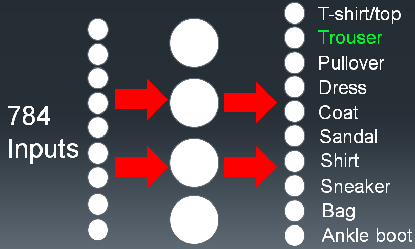
In the above design, we’re providing 784 inputs, one for each pixel in the (28x28) image. We’re receiving 10 different outputs, one for each unique class that our fashion objects can be classified as. The hidden layer can consists of any number of neurons and layers, depending on how deep or shallow you’d like your neural network to be. For deeper abstraction and higher processing results, such as with deep learning, you would generally include a larger number of hidden layers and neurons. For our purposes, a relatively shallow neural network will suffice.
Of course, neural networks are just one type of machine learning model that can be applied to image recognition and classification. We’ll actually be using several different machine learning algorithms to build models and compare their accuracy results. These include logistic regression, support vector machines, and boosted trees.
Let’s take a look at some of the accuracy results that can be achieved with a simple image recognition model as we’ve described above.
Preparing the Labels
To get started, let’s first convert the y labels for each image into a factor. This allows them to be unique classes across all of the image data. We can use the code shown below to do this.
1 | # Convert y-value to a factor. |
Additionally, let’s assign readable labels to the factor so that we can identify the category for each image, without having to lookup the numerical value for each predicted class.
1 | # Set labels. |
As you can see in the above code, we’ll limit our training data to just the first 10,000 images. In this manner, we can speed up the processing time to train our machine learning models. Depending on the speed of your computer, you may wish to train on the full dataset. Keep in mind, since we have labels for both the training and test set, you can combine the two and train on the entire dataset (70,000 images) for an additional boost in accuracy.
With the data setup, we can begin training. But first, let’s see what a baseline accuracy for the data would be without using any machine learning just yet.
Determining a Baseline Accuracy
Before training a machine learning model, it’s important to look at a baseline accuracy score of classifying the images without machine learning. In this manner, we can get a better idea on if our artificial intelligence machine learning model is actually learning anything, and thus, improving upon a non-machine learning algorithm approach.
A common metric for producing a baseline accuracy result is to simply guess. In this case, we can simply take the most frequently occurring class of fashion object, and just assume every image will be this class. After all, if we predict the most commonly occurring category for each image, we’ll have a slightly better chance of getting the predictions correct for each image, than guessing any of the other classes.
How Many Classes of Each Image Do We Have?
Since we want to find the most frequently occurring class of image, in order to calculate a simple baseline result, let’s see how many different image classes we actually have in our dataset.
1 | table(dataTrain$y) |
The above code results in the following table of machine learning image recognition classes (remember, we’re only looking at the first 10,000 images!):
1 | T-shirt/top Trouser Pullover Dress Coat Sandal Shirt |
We can see from the above table that Trouser is the most frequently occurring class of image. Therefore, if we always predict Trouser for each image in the dataset, we should have the best possible accuracy when completely guessing a class. This will be our baseline accuracy.
Baseline Accuracy
A baseline accuracy with this “guessing” metric can now be calculated by simply dividing the maximum number from the list of classes by the number of images in our training set.
1 | max(table(dataTrain$y)) / nrow(dataTrain) |
We end up with an accuracy of 0.1027 or 10.27%. This doesn’t seem so great, especially considering that we have 10 different categories of images. With 10 categories, guessing any particular category (on a fully balanced dataset) would give us an accuracy of about 10%. Naturally, since our dataset is indeed (mostly) balanced across the classes, this explains why our baseline accuracy is around 10%. We get a slight boost since there are a few more images of “Trouser” objects than any other type of image in the dataset.
Recall, we’re looking at the categories for only the first 10,000 images in the dataset. If you actually look at the classes for all 60,000 images in the training set, they are actually perfectly balanced across all categories! Each category in the entire dataset of training images has 6,000 images per category. The same applies to the test dataset as well, with 1,000 images balanced across each category.
Now that we have a baseline guessing accuracy of 10.27%, let’s see if machine learning image recognition can do better.
Results
For each machine learning model that we apply to our data, we’ll be using the following code to measure the accuracy results in a confusion matrix and overall accuracy. Recall, we’re only training on a 10,000 image subset of the data in order to obtain quicker results.
1 | # Train. |
The confusion matrix appears as follows.
1 | Confusion Matrix and Statistics |
With a confusion matrix, optimal accuracies will show as a diagonal line of large values from the upper-left down to the bottom-right of prediction categories. For each reference class, you want to see the highest value for the same class prediction.
For the above confusion matrix (based upon the results of a gradient boosting machine model), the accuracy is 90%.
Let’s take a look at our results.
Logistic Regression
81.3% / 74.8%
Using a machine learning model of boosted logistic regression, we can calculate an accuracy with the following code.
1 | fit <- train(y ~ ., data=dataTrain, method = 'LogitBoost', trControl = trainctrl) |
Boosted Trees (GBM / XGBoost)
90.1% / 85.3%
With boosted trees, we get the following result.
1 | fit <- train(y ~ ., data=dataTrain, method = 'gbm', trControl = trainctrl) |
Neural Network / Multinomial Regression
83.5% / 78.3%
With a multinomial regression, we get the following result.
1 | fit <- train(y ~ ., data=dataTrain, method = 'multinom', trControl = trainctrl, MaxNWts = 10000) |
Support Vector Machine (SVM)
91.2% / 87.2%
With a support vector machine, we get the following result.
1 | fit <- train(y ~ ., data=dataTrain, method = 'svmRadial', trControl = trainctrl) |
Are We Learning Anything Yet?
From the machine learning image recognition accuracies shown above, we can see that the machine learning models are certainly achieving far better results than our baseline “guessing” model was achieving. The best model that we’ve trained on just 10,000 images (an SVM) has scored an accuracy of 91% on the training set and 87% on the test set. If you compare this to our baseline accuracy (the “guessing” model) which simply predict the most frequently occurring category (Trouser) for every image, we achieved an accuracy of only 10%.
Our machine learning prediction models for image recognition have a large boost in accuracy over our baseline model, proving that our models are indeed better than simply guessing.
In fact, let’s see how our model does on real-time images of fashion items from the web.
Testing the Model on Real Fashion Images
To test our model out on real images, we can perform an online image search for the fashion category that we’d like to test. For example, let’s try a dress.
Resizing the Image for Classification
Since our machine learning model was trained on images of size 28x28 pixels, we just need to resize the image before we try processing it with our artificial intelligence machine learning image recognition model. To do this, we can simply download the image and edit it in any paint program to resize it to the correct dimensions. Keep in mind that resizing an image to a fixed resolution of 28x28 pixels will likely distort the aspect ratio and image quality, which can cause classification predictions to be less reliable. However, it still gives an idea of how image recognition machine learning algorithms work.
We’ll also need to color the background black, in addition to resizing to 28x28 pixels. After this pre-processing is complete, we can load the image into our model. The image appears as shown below.

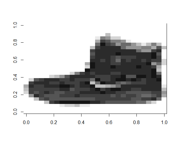
Since the above image is a close-up view of the 28x28 pixel image (which is quite small to see, although the AI has no problem classifying it!), below is the actual image in its true resolution. You can get an idea of just how small these images are, that the AI is still able to successfully classify!

It’s quite small, but our machine learning model was trained to handle it. Let’s run the image through our image recognition model and see what category our AI identifies the image as.
Loading the Image and Classifying It
We can load and classify the image with the following code.
1 | # Helper for running a trained model against actual 28x28 PNG images. |
The above helper methods simply loads the png image. It then displays the image, so we can see what it looks like. It then converts the bytes within the image to the format required by our model (gray-scale with 784 total integer values). Finally, it calls the predict method to classify the image as a particular type of fashion item.
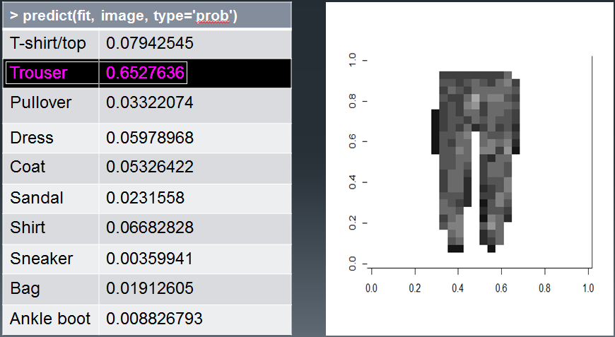
The Final Result on our Test Image
Finally, we can run the helper method to load and classify our image. Let’s see how it does.
1 | runTest('data/test/dress-28x28.png', fit) |
The output from the above test is shown below.
1 | [1] Dress |
Success!
Checking machine learning models on real live test data is a convenient and human-friendly way to demonstrate a sense of accuracy about your machine learning model. Of course, the actual statistical accuracies are much better, but visual demonstrations can be helpful nonetheless. Visual tests, along with statistical accuracy measurements are methods for showing that our machine learning model has actually learned with a degree of accuracy.
Another way that we can show evidence that our machine learning models are predicting better results, and actually learning, is to plot a learning curve.
The Learning Curve
Learning curves are a way of viewing accuracy predictions over increasingly larger sets of data. You can build a learning curve by training and running a machine learning model over gradually increasing sets of data. The more data that you train your machine learning model on, the less accurate you would expect your training accuracy to be and the more accurate you would expect your cross-validation or test set to be.
Consider the idea in detail. If you train a model on just 1 image, it should easily be able to learn to classify it correctly. After all, it’s just 1 image with 1 category. Easy. This would result in 100% accuracy for 1 image. Now, run this same model on a test image with a different category. It will most likely predict the same category for the single training image for this test image. After all, the only image it’s ever seen was the single training image. Therefore, it will likely predict that same category for the test image as well. This results in an accuracy of 0%. In this scenario, the two accuracies are as far apart as possible (100% versus 0%).
Next, consider the same idea with a slightly larger dataset of 10 images. The machine learning model should still obtain a very high accuracy, since it only needs to learn 10 different images. Now run this model against a test set. You would expect it to still do poorly, although it might achieve a slightly better accuracy than 0% (as we saw when only training on 1 image). This is because the model will have now seen 10 different images, giving it a better chance of at least getting 1 image correct in the test set. This might show up as an accuracy of 99% versus 1% or similar.
In general, the more training data that a machine learning model has exposure to, the worse the training accuracy and the better the test accuracy. It becomes harder for the model to learn over more training data. However, the range of data allows it to generalize better on new images that it hasn’t seen before. At a certain point, the two accuracies begin to converge (or at least, come close to doing so).
In this manner, a learning curve can show us whether our models are actually learning from the data and obtaining better accuracies on the cross-validation or test sets over increasingly larger sets of data. We can also get an idea of whether more data will make our models better!
Our Fashion Learning Curve
To demonstrate that our machine learning image recognition model is actually learning, we can plot a learning curve of our data over increasingly larger training sets. We’ll plot the training set accuracy and a test set accuracy against it. We can use training set sizes starting from just 1,000 images all the way up to 60,000 images. Doing so, produces the following learning curve.
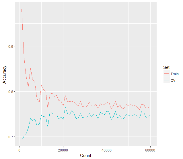
You can clearly see, just as we’ve described above, that the learning curve consists of two lines arcing downwards and towards the right, appearing to eventually converge. The training set accuracy begins almost at 100% and the test set accuracy much lower around 60% or less. As more training data is fed to the machine learning model, our training accuracy quickly drops to around 80%, while the test set accuracy increasingly improves towards 75% and higher.
If we plot a trend line across the training and test sets, it becomes even more apparent how the accuracy levels begin to converge around 75% after around 55,000 training images.
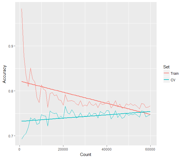
You can see from the learning curve plots, that after 60,000 images have been used for training, both the training set and the test set appear to converge towards about 78% accuracy. If we feed the model more image data to train upon, it appears that our model may not get much better than this. This is the primary benefit of using a learning curve, in that it can tells us whether we should spend time locating more training data, or perhaps spend our time fine-tuning our model instead and feature list instead.
Building a Learning Curve
Now that we know what a learning curve can do, let’s see how to construct one. All that we need to do is to subset our training data into gradually larger sets of data, training our machine learning image recognition model each time on the new sets of data. We can then plot the accuracy result of the training and test set for each iteration of data.
To build a learning curve from our image recognition fashion dataset, we just need to iterate over a loop, training our model each time on a larger set of data. We can do this with the code shown below.
1 | library(reshape2) |
In the above code, notice that we simply invoke a for loop to iterate over our data-set 30 times. Each iteration increases the number of records that we train with by 1000. In this manner, our model trains on ever increasing rows of data. This allows us to draw a learning curve chart with the accuracy on the y-axis and the data-set size on the x-axis.
Learning curves can be incredibly powerful for analyzing the performance of your machine learning models. For example, they can indicate bias and variance within your model, as well as the success rates of learning over larger data-sets. For these reasons, it’s important to understand and consider the use of learning curves when validating artificial intelligence machine learning models.
Download @ GitHub
The source code for this project is available on GitHub.
About the Author
This article was written by Kory Becker, software developer and architect, skilled in a range of technologies, including web application development, artificial intelligence, machine learning, and data science.
Sponsor Me