Introduction
Are you preparing to take a quantum computing certification? Learning about quantum computing and the topics of quantum circuits, qubit gates, Bloch spheres, and the Qiskit SDK are part of the overall technology for being certified as a quantum computing developer. As quantum computing is gaining increasing traction amongst companies competing to be the first to leverage this powerful technology, it has the potential to revolutionize computing and become a major technology tool for developers, engineers, and hiring within companies.
A quantum computing certificate not only demonstrates proficiency with quantum computing and programming a quantum computer, but it also helps those hiring for classical programming and technical leadership roles to recognize certified individuals as forward-thinking and leading-edge technologists and engineers, willing to adapt to future technologies and skillsets. This is especially important for an emerging technology, such as quantum computing, which has not yet achieved production quality implementation in industry. However, as quantum computers mature, industries and the computing workforce will most certainly implement these powerful computers within their organizations and require a workforce knowledgeable in the field.
This article is a guide through the IBM Professional Certification Program for Quantum Computing, also called Fundamentals of Quantum Computation using Qiskit v0.2X Developer (C1000-112, A1000-112, IBM Quantum).

Passing the certification exam earns you the following certificate.
In this article, we’ll walk through the set of topics including how to define, execute, and visualize quantum circuits using Qiskit. We’ll also review single and multi-qubit gates and their associated rotations on the Bloch sphere. Most importantly, we’ll review how to use the Qiskit SDK to implement quantum computing applications and begin programming your own quantum computing programs.
We’ll be following through the study guide topics as we prepare to take the Qiskit developer certification exam by IBM.
Table of Contents
- My Personal Experience Taking the Certification Exam
- IBM Quantum Composer
- Creating Logic Gates with IBM Quantum Composer
- Measuring Outputs in the IBM Quantum Composer
- Predicting Output From Quantum Circuits
- X Gate (NOT)
- Y Gate
- CNOT Gate (AND)
- NAND Gate
- XOR Gate
- OR Gate
- Quantum Gate Icons
- Initializing Qubits Using State Vectors
- Two Methods to Load a State Vector
- Calculating the Depth of a Quantum Circuit
- Drawing a Quantum Circuit
- Plotting a Bloch Sphere
- Initializing a Qubit in Superposition
- Initializing a Qubit to a Variable Degree
- Collapsing a Superposition
- Quantum Circuit Identities
- Creating an X-gate from HZH
- Entanglement
- Bell States
- Swapping Two Qubits
- Swapping N Qubits
- GHZ State
- A Unitary Matrix for a Quantum Circuit
- Phase Kickback
- Barrier Operations
- Qiskit Version
- Running on IBMQ
- Monitoring the Status of a Job
- Visualizing Quantum Circuits
- OpenQASM
- Plotting Gate Maps and Error Rates
- Creating Phase on Qubits
- Fidelity
- Density Matrix
- Creating Custom Gates
- Composing Circuits from Other Circuits
- Decomposing a Quantum Circuit
- Adding Controls to Gates
My Personal Experience Taking the Certification Exam
My own story begins with having worked with quantum computing in Qiskit and Python for about 2 years prior to the certification becoming available. I had already been passionate about quantum computing and its potential. However, once IBM had released an official certification process and exam, I jumped at the opportunity to gain professional credibility and skill in quantum computing, especially with regard to programming.
I truly believe quantum computing has the amazing potential to revolutionize the way computers are used. Programmers of today may very well find the need to up-skill to keep on track with the ever changing world of technology. We’ve already seen how quickly things can change with artificial intelligence and machine learning. We may very well be seeing the beginning of the quantum computing revolution as well.
With this in mind, the certification made perfect sense to prove skill in quantum computing programming.
This article follows through a list of topics that are required for passing the exam. You’ll want to study the material below, including the links in the references section at the end of this article. Once you feel that you are prepared, you can register to take the IBM Professional Certification exam.
Details About the Exam
The exam, C1000-112 Fundamentals of Quantum Computation Using Qiskit v0.2X Developer, consists of 60 questions. You are allotted 90 minutes to complete it and you are required to pass 44/60 questions (73%) in order to pass and obtain the certification.
Three types of the exam exist.
The first type is a free sample test with 20 questions, similar to what you can expect from the full exam.
The second type is a web-based assessment (A1000-112), which I would highly recommend taking, prior to the official proctored exam. The web assessment version is $30 and is offered online with a graded score by section. You are allotted 90 minutes to complete the web assessment version of the exam with a results section providing a pass/fail score, along with percentages of correct answers per section. Note, individual questions are not labeled as correct/incorrect, so you would need to estimate by the labeled category, which questions you may have gotten wrong.
The third type is the proctored certification exam. This exam is $200 and is proctored online or in-facility by Pearson Vue. You’ll schedule a date and time to take the exam. I was very impressed with the available times, which run nearly 24-hours a day and may be scheduled as soon as one hour from now. Before taking the exam, you’ll check-in to an online portal, which includes taking pictures of your desk space and government issued ID using your mobile phone (through a link that the exam site will provide to you). After signing in, you may then access the exam, which feels very similar to the assessment web-based version. One difference is that your screen video and sound will be recorded during the exam, as per the proctored process.
After successfully passing the exam, you’ll receive an IBM Associate Certified Developer in Quantum Computation using Qiskit v0.2X certification. You can view the official badge and license issued by IBM Professional Certification.
An IBM Qiskit Developer is an individual who understands fundamental quantum computing concepts and is able to express them using the Qiskit open source software development kit (SDK). They have experience using the Qiskit SDK from the Python programming language to create and execute quantum computing programs on IBM Quantum computers and simulators. This individual is able to perform these tasks with little to no assistance from product documentation.
Let’s get started with the topics to study!
Composing Quantum Circuits on the Web
The IBM Quantum Composer is a graphical web-based application for visualizing and creating quantum circuits. It allows you to drag and drop quantum computing circuit controls (i.e., operations) to build quantum circuits and execute them in a simulator or on a real quantum computer at IBM.
Let’s take a quick look at how to create some basic logical gates using qubits (quantum computing bits) and the IBM Quantum Composer application.
Creating Logic Gates with IBM Quantum Composer
Quantum computing bits are called qubits. Just like a classical bit in a computer, qubits can represent the value of 0 or 1. However, on a quantum computer, qubits can be placed into superposition, allowing them to hold a value of 0 and 1 simultaneously or any value in between.
When we are not placing qubits into superposition, qubits will behave in the same manner as classical bits, resulting in a direct measurement of either 0 or 1. This makes it easy for us to start experimenting with qubits and the IBM Quantum Composer by creating logical gates to perform operations on a quantum circuit.
Some of the most basic gates include NOT, AND, OR, NAND, and XOR. Let’s walk through how to create each of these logic gates in quantum computing with qubits and the IBM Quantum Composer. We’ll also see how we can recreate each of these logical gates on both the IBM Quantum Composer and in Python with Qiskit.
We’ll start with the simplest gates, which are the set of Pauli gates (X, Y, Z).
X Gate (NOT)
The most simplest of the logic gates is the Pauli X-gate, also called the NOT gate. This gate simply inverts the value of a qubit from 0 to 1 or 1 to 0. Due to this simple inversion of the value, the Pauli X-gate is often referred to as a bit-flip, since it “flips the bits” of the affected qubits.
1 | NOT |
See the example.
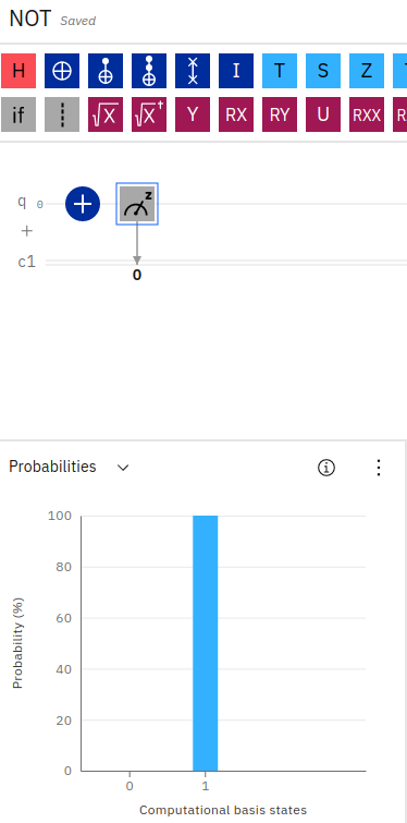
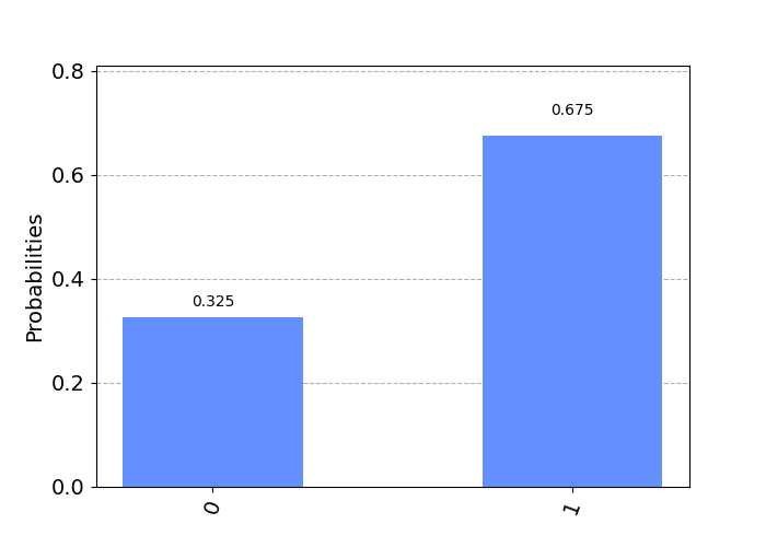
In the above screenshot, we can see how a single X-gate is applied to a qubit, followed by a measurement instruction. The resulting probabilities in the blue bar chart show 100% probability of the qubit measuring as a 1.
We can create this simple circuit in the IBM Quantum Composer by dragging a NOT gate, indicated by the plus sign with a circle onto a single qubit, followed by a measurement icon.
Since qubits are initialized with a default state of 0, after applying the NOT gate our measurement of the qubit results in a value of 1.
We can see an example of this using Python Qiskit in the example shown below.
1 | from qiskit import qiskit, QuantumCircuit |
In the above example, we create a QuantumCircuit with 1 qubit and 1 classical bit. We apply the Pauli X-gate to invert the qubit from a default value of 0 to a value of 1, and finally measure the resulting qubit in a classical register. We run the circuit in the simulator and print the results, as shown below.
1 | {'1': 1024} |
If we similarly apply two X-gates in succession, we can see the qubit flip from 1 to 0.
1 | {'0': 1024} |
Measuring Outputs in the IBM Quantum Composer
Since we’ve just introduced the X-gate for inverting a qubit, this is a convenient time just to highlight how to read the IBM Quantum Composer probability bar chart to understand output from a quantum circuit.
Recall from the example above that the blue bar chart shows probabilities for 0 and 1 for a single qubit. In this case, the result was a 100% probability of measuring a 1 (or simply, a value of 1).
Output probabilities for a quantum circuit are shown in this bar chart on IBM Quantum Composer. If two qubits were used in the circuit, the chart would contain tick marks for 00, 01, 10, 11. Similarly, for three qubits, you would have 000, 001, 010, 011, 100, 101, 110, 111. In this manner, you can see which outcome that the qubit would result in after applying the series of quantum gates.
You can also step through the changes in output to the qubits by using the IBM Quantum Composer Inspector tool. In the file menu, select Inspect. You can then play through each logical gate execution across the quantum circuit and see changes step by step.
It’s important to note that the bits displayed in the bar chart are read from right to left, corresponding to each qubit in the circuit (from 0 .. i). For example, if your quantum circuit has two qubits (q0, q1) with the first qubit in a state of 1 (q0=1, q1=0) the output chart would show 01 = 1. Reading from the right to the left, q0 has a value of 1 and q1 has a value of 0 and this result (01) has 100% probability - meaning the circuit has a resulting value of 01.
In the above screenshot, you can see how the quantum circuit contains three qubits. The first two qubits have a default value of 0 and the third qubit is inverted to have a value of 1. The resulting output probability in IBM Quantum Composer is shown as 100 having 100% probability. Reading from right to left, q0=0, q1=0, q2=1.
Now that we understand how to read the output from a quantum circuit in IBM Quantum Composer, let’s see how to predict output from any quantum circuit.
Predicting Output from Quantum Circuits
Quantum circuits are built using qubits, which correspond to any value between 0 and 1. When not in superposition, a qubit will output an explicit value of 0 or 1. However, when in superposition, a qubit will hold the value of both 0 and 1 simultaneously. For this reason, it can be a bit challenging to predict the output of a quantum circuit, especially those containing qubits in superposition.
Let’s take a look at a couple of example quantum computing circuits and see how to predict their output. We’ll start with a quantum circuit containing a single qubit.
Predicting the Output From One Qubit
Suppose that we have a quantum circuit consisting of a single qubit. If the qubit is not in superposition, it’s easy to predict its value as 0 or 1.
1 | qc = QuantumCircuit(1, 1) |
All measurements (shots) on this circuit will result in a 0. If we were to apply the bit-flip operator (X-Gate), the value would be 1. The result from the above circuit is shown below.
1 | {'0': 1000} |
Let’s place the qubit into superposition and predict the results. Since the qubit will now hold a value of both 0 and 1, we can expect the result to be split 50/50, that is: {'0': 500, '1': 500}. Let’s see the result.
1 | qc = QuantumCircuit(1, 1) |
Sure enough, the result is split evenly as shown below.
1 | {'0': 490, '1': 510} |
Predicting the Output From Two Qubits
Let’s take it a step further and use two qubits. It’s important to be familiar with predicting quantum circuit measurement outputs in order to accurately build and analyze quantum computing circuits (especially so for the certification exam!).
1 | qc = QuantumCircuit(2, 2) |
What do you expect the result to be from the above circuit? Since we have two qubits (no superposition applied), we expect the result to be {'00': 1000}. Let’s see.
1 | `{'00': 1000}` |
Now, what if we bit-flip one of the qubits?
1 | qc = QuantumCircuit(2, 2) |
We’ve inverted the value of the second qubit. What do you expect the result to be? Since the convention is to show output from right to left (with q0 being the right-most value), we should expect to see the result as {'10': 1000}.
1 | `{'10': 1000}` |
Next, let’s place a qubit in superposition. Since that qubit can now result in a value of both 0 and 1, we expect to get simultaneous values for all possible combinations of that qubit in superposition, along with the static qubit. That is, we can expect {'00': 500, '10': 500}. We’re expecting the second qubit (the left-most one, that we’ve placed into superposition) to hold a possible value of both 0 and 1, while the first qubit (the right-most one) stays fixed at 0.
1 | qc = QuantumCircuit(2, 2) |
Sure enough, you can see below how the first qubit stays fixed at 0 while the second has both 0 and 1.
1 | {'00': 483, '10': 517} |
What if we place both qubits into superposition? Well, now we’re going to get all possibilities for two qubits 00, 01, 10, 11 each split into 4 equal results.
1 | {'01': 254, '00': 269, '11': 231, '10': 246} |
Predicting the Output From Three Qubits
Let’s see one more example, this time using 3 qubits. To keep things reasonable, we will only place one of the qubits in superposition. What do you expect the circuit below to output?
1 | qc = QuantumCircuit(3, 3) |
If you expect the output to have two possible combinations, evenly split, then you’re correct! We should see {'010: 500, '011': 500}. Why? Because the first qubit (the right-most) is placed into superposition, so it will have both a 0 and 1. The second qubit (the middle) is bit-flipped to 1 and will remain fixed at that value. The third qubit (the left-most) is left as 0. This leaves us with 010 and 011.
1 | {'010': 512, '011': 488} |
While we could extend this section by placing all qubits into superposition qc.h(range(3)), you can imagine how the output results can grow exponentially according to the number of qubits in superposition (it’s also probably more than enough for the certification exam!).
By the way, if you were curious about the result of 3 qubits in superposition, indeed it would result in an equal split of 2^3 possibilities {'110': 113, '111': 108, '001': 134, '100': 116, '011': 145, '010': 141, '000': 111, '101': 132}.
Thus, that’s enough measurement for now. Let’s move on to building the next quantum gate example - this time, operating on two qubits instead of just one, the Y-Gate!
Y Gate
Another basic single-qubit Pauli gate is the Y-gate. The Y-gate is equivalent to a bit value and phase flip in one operation. That is, while the X-gate only flipped the bit value for the qubit from 0 to 1 or from 1 to 0, the Y-gate not only flips the value, but also flips the phase from +1 to -1 or from -1 to +1.
When the qubit is not in superposition with a Hadamard gate, the Y-gate looks just like an X-gate, simply flipping the classical value from 0 to 1. However, when a Hadamard gate is used first, the Y-gate has the additional effect of flipping the phase.
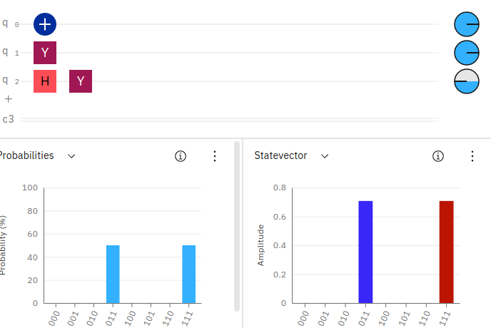
You can see in the circuit above, we’ve added 3 qubits. The first qubit simply applies an X-gate, which flips its value from 0 to 1. The second qubit applies a Y-gate without superposition, again flipping the value from 0 to 1. However, the third qubit applies a superposition via the Hadamard gate and then applies a Y-gate, flipping the value from 0 to 1 and also flipping the phase to -1 (as can be seen in the phase disk along the right-most side of the qubit line.
CNOT Gate (AND)
While the NOT gate in the above example operated on a single qubit, the next set of gates operate on two qubits. The AND gate takes two input qubits and if both hold a value of 1, then a resulting qubit will be set to 1. If either of the input qubits are 0, the resulting qubit will be 0.
1 | AND |
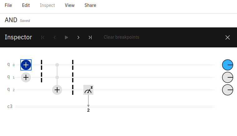
An AND gate can be easily constructed using a Toffoli gate also called a “CCNOT gate” (i.e., double-controlled condition NOT gate) or “AND gate”. A Toffoli gate simply takes two input qubits and flips the value of a resulting qubit if the two inputs hold a value of 1. This effectively performs an AND operation.
See the example.
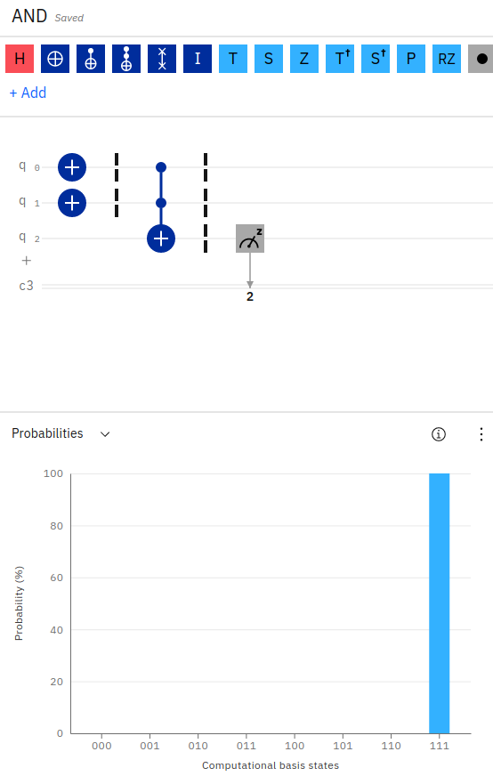
As you can see in the above quantum circuit in the IBM Quantum Composer, we’ve initialized two qubits to have a value of 1 (by applying the X-gate on each qubit, inverting their default values from 0 to 1). We then apply a Toffoli gate (CCNOT) gate on the two input qubits with an output stored in a third qubit. Since the two input qubits hold a value of 1, the resulting output bit will be flipped from 0 to 1.
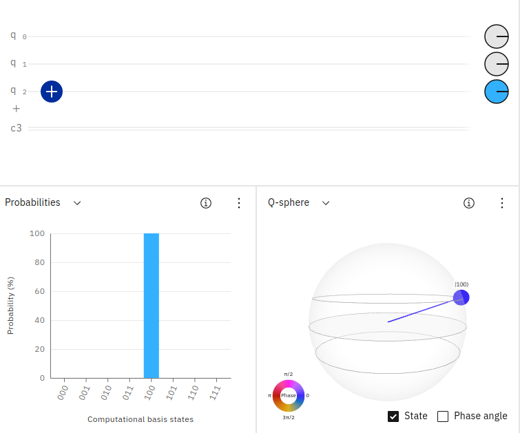
Notice in the probability output, the IBM Quantum Composer is showing 100% probability for the result of 111. Reading the output from right to left, q0=1, q1=1, q2=1. This makes sense since we’ve initialized the first two qubits with a value of 1 (by inverting their values using the X-gate) and we’ve applied a Toffoli gate across those two qubits, storing the result in the third qubit. Since the Toffoli gate is an AND operation, and the two inputs were 1, 1 AND 1 equals 1 - hence the third qubit has a value of 1.
Just to prove this a bit better, here an example of running the same quantum circuit with an AND gate with the first qubit having a value of 1 and the second qubit having a value of 0 (q0=1, q1=0, q2=0).
Since 1 AND 0 equals 0, the resulting probability output (reading right to left) shows 100% probability of measuring 001.
We can write the Python Qiskit code for an AND gate with the following example below.
1 | def and_gate(a, b): |
NAND Gate
Following from the above example, we can implement a NAND gate (NOT AND) using nearly the same circuit as the above example for AND and applying a NOT operator on the result.
1 | NAND |
See the example.
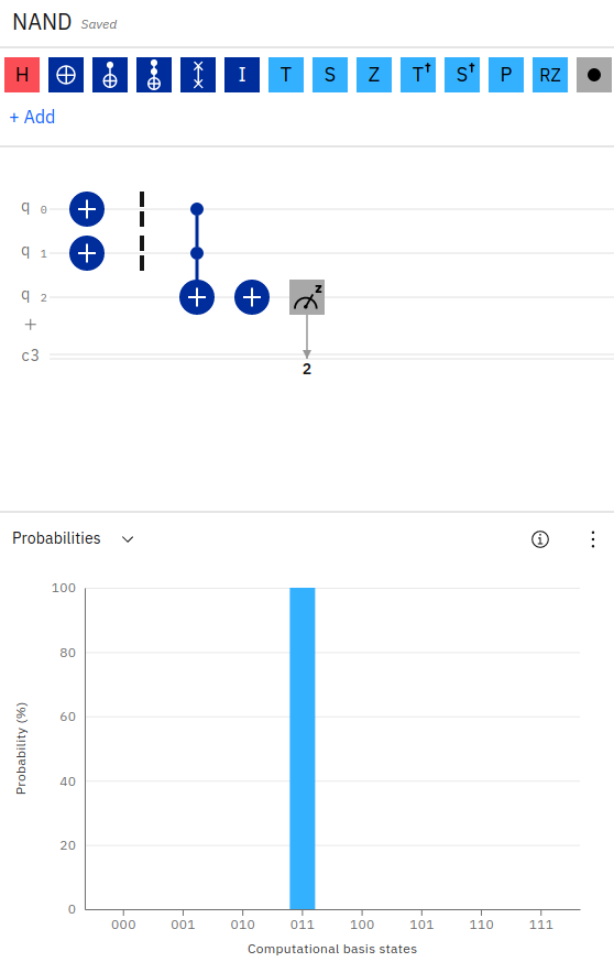
Notice, we’ve applied an X-gate to the first two input qubits. We’ve then applied a Toffoli (AND) gate across the first two inputs, storing the result of the operation in the third qubit. Finally, to implement a NAND, we apply an X-gate to the output qubit, flipping its value.
We can see in the output probability that the result is 011 (q0=1, q1=1, q2=0) since 1 NOT AND 1 equals 0.
1 | def nand(a, b): |
Notice, in the above code for NAND, we’re simply using the qc.ccx() operator to perform a Toffoli gate on the first two qubits (q0, q1) and storing the result in the third qubit (q2). We then apply an X-gate to the third qubit (q2) to create our result.
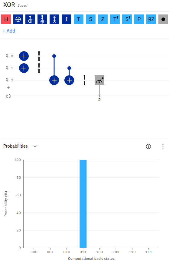
XOR Gate
The XOR gate (or exclusive OR) can be created by using a CX-gate, also called a “controlled NOT gate”. This gate takes an input qubit (called the control bit) and an output qubit. The output qubit will be inverted only if the input qubit has a value of 1. If the input has a value of 0, no change is made on the output.
Using the CX-gate, we can create an XOR operation by placing two CX-gates in the circuit, with one on each input qubit, and storing the result on the same output qubit. Since the CX-gate will flip the output qubit if its input has a value of 1, the first qubit CX-gate operation will set the output to 1 if the input was 1. So far, so good. The second CX-gate will set the output to the opposite if the second input was 1. So, if the first input was a 0 the output is currently a 0 and thus, will be set to a 1 (if the second qubit is 1). Likewise, if the first input was a 1 and the output is currently a 1, the second qubit holding a value of 1 will flip the output again back to 0. This makes sense, since 1 XOR 1 equals 0, and 0 XOR 1 equals 1.
1 | XOR |
See the example.
We can implement the XOR gate in Python Qiskit with the following code below.
1 | def xor(a, b): |
Notice in the above example, we apply a qc.cx() or (controlled NOT) on each qubit, storing the result in the third qubit. We then measure the result.
OR Gate
Our final logic gate example is the OR gate. While the AND gate compares the two input qubits for having a value of 1 in order for the output to have a value of 1, the OR gate will set the output to 1 if either of the two inputs are 1.
The OR gate is implemented on a quantum circuit by using two CX-gates (conditional NOT) followed by a Toffoli gate.
1 | OR |
See the example.
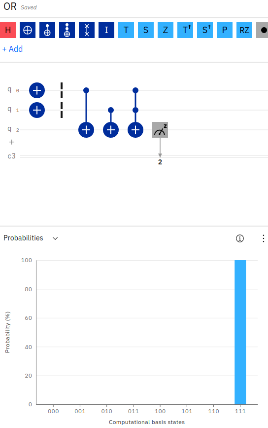
The OR logic gate is slightly more complex than our prior examples, in that it contains an additional logical gate. The OR circuit combines the conditional NOT operator (CX) with a Toffoli operator (CCX) to “AND” the result.
Notice in the above screenshot, the OR gate appears very similar to the XOR gate. We first apply a conditional NOT (CX) operator to each of the input qubits (q0, q1), storing the result in the third qubit (q2). However, we then apply a Toffoli gate (CCX) across the first two inputs again, and store the result in the third qubit. This effectively applies an XOR operation first, and then to handle the case for when the two inputs are both 1, the Toffoli gate flips the output accordingly.
That is, to implement the OR gate, if the first qubit is 1, we flip the output qubit to 1. Otherwise, we leave it as 0. If the second qubit is 1, we flip the result bit again (to 0 if the first was 1, or to 1 if the first was 0). Otherwise, we leave the output qubit as-is. Finally, if both input qubits are 1, we flip the result qubit one more time.
This is better described by taking a look at the Python Qiskit source code.
1 | def or_gate(a, b): |
Notice in the above code how we’ve chained together the two CX operators, followed by the CCX. For example, if q0=0 and q1=1, the first CX will leave the output as 0. The second CX will flip the output to 1. The final CCX will leave the output as 1. Hence, 0 OR 1 equals 1. The real test comes from the case of q0=1 and q1=1, in which case the first CX will flip the output to 1, the second CX will flip the output back to 0, and the CCX will flip it one more time back to 1 (since both inputs are 1). Hence, 1 OR 1 equals 1.
The Python Qiskit code for the logic gate examples above are available here.
Quantum Gate Icons
There are convention icons used for visualizing the various quantum gates on a circuit. For example, the ‘+’ symbol is used to indicate an X-Gate and most gates are indicated by the first letter in their name (Y, Z, S, T, P, U).
![]()
The above image displays icons for quantum gates, with the symbols being self-explanatory, with the exception of ‘+’ for an X-Gate, meter for a measurement gate, and two vertical lines (|) for a barrier.
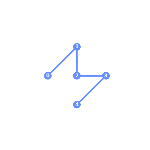
While some gates are more obvious than others, such as ‘Y’ for a Y-gate and ‘H’ for an H-Gate, others use symbols that may be less obvious, especially when spanning across multiple qubits (controlled gates), as shown below.
![]()
The above icons show the following gates, from left to right.
1 | Swap |
Note, Z-gates are indicated by a single dot while swap gates are indicated by X.
Initializing Qubits Using State Vectors
In the first example of using quantum computing logic gates with Qiskit and the IBM Quantum Composer, we used an X-Gate to execute a quantum circuit on a quantum computer simulator and counted the number of shots that resulted in a measurement of 0 or 1. Quantum circuits can be executed in Qiskit using the simulator and shot count, as demonstrated in that example. However, we can also initialize qubits using a state vector and apply the simulator to obtain the result. This allows us to set up a quantum circuit without running an actual gate on it yet.
The below code creates a quantum circuit, just as we’ve performed in the original X-gate example, but uses a state vector to initialize the qubit in a state of 0. We can then apply the X-gate on the qubit and measure the result.
1 | from qiskit import QuantumCircuit, assemble, Aer |
In the above example, we create a QuantumCircuit with 1 qubit and 1 classical bit. Next, we initialize a state vector for our qubit to place it in a default value of 0. The state vector is simply [1, 0] (The second value indicates the qubit value, which is 0). We then apply an X-gate to the qubit, which inverts the value from 0 to 1. Finally, we measure the resulting qubit value. To test this example without actually running in a quantum computer simulator, we’re using the aer_simulator, which mimics a real quantum computer backend, including error rates. We save the state vector after applying the NOT operation and then compile and execute the circuit in our simulator.
The last line prints the results of the circuit. We can see how our initial state was [1, 0] and after applying the X-gate, our state resulted in [0, 1].
1 | [1, 0] |
Similarly, we can initialize our qubit in a state of [0, 1] and apply the X-gate to obtain a result of [1, 0].
1 | [0, 1] |
Two Methods to Load a Statevector
Qiskit state vectors can be retrieved using two methods. These include the Statevector constructor object by evolving the resulting vector, and the BasicAer or Aer simulator “statevector” method.
First, let’s see an example of the Statevector object.
1 | from qiskit import qiskit, execute, QuantumCircuit, BasicAer |
In the above code, we’ve evolved a random quantum circuit to obtain a state vector. We can then plot the resulting state vector visualization by directly calling the draw method on the state vector object (and passing in the desired plot: “city”, “paulivec”, “hinton”, “bloch”). We can also plot visualizations using the plot state methods and passing in the statevector result.
Next, let’s load a state vector from the simulator.
1 | backend = BasicAer.get_backend('statevector_simulator') |
Notice, this time we are not able to call a “draw” method on the resulting state vector, since we’re not getting back an instantiated “Statevector” object. Instead, we can only use the plot methods. Attempts to call the “draw” method directly on a get_backend('statevector_simulator') result, will display the following error, as shown below.
1 | sv.draw('city') |
1 | --------------------------------------------------------------------------- |
Calculating the Depth of a Quantum Circuit
The depth of a quantum circuit is defined as the number of quantum gates that executed along the longest path in the circuit. Each quantum gate that is executed (with the exception of barriers) adds +1 to the total depth.
Let’s take a look at an example of how to calculate the depth of a quantum circuit in Qiskit.
Example Depth 2
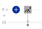
In the above example, we have a simple X-gate applied to a single qubit, followed by a measurement operation. To calculate the depth of this circuit, we simply count each gate. Since there are two gates, the depth of this circuit equals 2.
1 | Depth 2 |
We can confirm this with the following Python Qiskit code example.
1 | from qiskit import QuantumCircuit |
The above example prints 2. Let’s take a look at a second example.
Example Depth 4
In this example, from the OR logical gate, we’re executing a longer list of quantum gates on the circuit. Just as we performed in the first example for calculating the depth, we add +1 for each quantum operation. However, there is one additional rule to keep in mind.
Conditional NOT gates (CX, CCX) are special.
Since multi-qubit quantum gates that take inputs and an output affect multiple qubits, we calculate the depth for this operation by adding +1 to each of the inputs and then take the greater of the depths so far for the input qubits (not including this step) and add +1 to the result.
For example, if the depth for q0=3 and the depth for q1=1 and we apply a CX(q0, q1), we add +1 to the depth of q0 to make q0=4. To determine the depth of q1 we take the greater of q0=3 or q1=1, and since q0 is greater, the depth for q1=3+1=4.
Let’s walk through a second example.
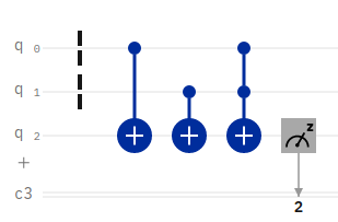
1 | Depth 4 |
Example Depth 5
As a final example, we’ll expand on the above OR gate by providing an input of q0=1, q1=0. This additional X-gate will affect the overall depth of our quantum circuit, as shown below.
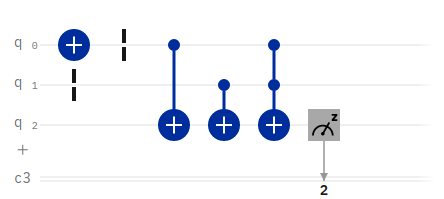
1 | Depth 5 |
The above example depth of 5 can be proven by taking the Python Qiskit code for the OR circuit shown earlier in this article and adding a command print(qc.depth()) after the measure command.
1 | from qiskit import QuantumCircuit |
Notice, when we calculate the depth for the quantum circuit in Qiskit above, we do not include the barrier operations, as they do not increase the total depth count.
Example Depth 4, But More Gates
Let’s see one more example of how to calculate and determine the depth of a quantum circuit in Qiskit. This time, our circuit has 5 gates, and yet the depth for the overall circuit is only 4. Let’s see how to calculate this.
1 | Depth 4 |
We can confirm the above calculation for the depth of the quantum circuit using Python Qiskit code as shown below.
1 | from qiskit import QuantumCircuit |
Notice, in the above code, even though we’re using 5 quantum operations, the total depth of the circuit in the longest path of execution is 4.
Drawing a Quantum Circuit
Visualizing a quantum circuit is a fairly easy process in Qiskit. We can simply use the qc.draw() command to draw a quantum circuit as a graphic. We can additionally print a QuantumCircuit to the console in plain text. Both operations are shown below.
1 | qc = QuantumCircuit(2, 2) |
The above example is from the qc.draw() command. We can also print a QuantumCircuit to display it in ASCII format, as shown below.
1 | ┌───┐ |
Drawing Types for Quantum Circuits
Several formats are available for drawing quantum circuits in Qiskit, with the default option being text. Available options include: text, mpl, latex, latex_source.
Providing an invalid drawing output type will result in the following error:
1 | VisualizationError: 'Invalid output type dfd selected. The only valid choices are text, latex, latex_source, and mpl' |
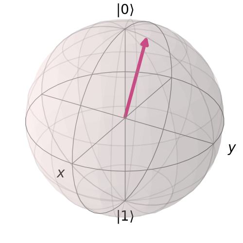
Plotting a Bloch Sphere
Since a qubit can have a value that corresponds to varying forms of axis, it can be helpful to visualize a qubit using a Bloch sphere. This allows a visualization of the various operations that may be applied to the qubit and their resulting effect.
A tool is available for experimenting with applying operations to a qubit and visualizing the resulting Bloch sphere.
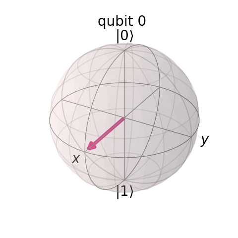
To generate and draw a Bloch sphere for a qubit in Python Qiskit, the follow code can be used.
1 | from qiskit import QuantumCircuit, qiskit, Aer, assemble |
Notice in the above code, we first execute the circuit in order to obtain the resulting state of the qubit. We then obtain the resulting state vector for the qubit and plot it on the multivector Bloch sphere. Finally, we save the Figure object to a PNG file.
Note, in the above code, we’ve used the method plot_bloch_multivector and passed in the output state from a job’s get_statevector(). As an alternative, we can also plot a bloch sphere by initializing a “Statevector” object and calling the Statevector draw method with the parameter “bloch”.
Now that we’ve seen how to visualize a qubit and its current state vector, let’s see how to initialize a qubit into varying states for X, Y, Z values.
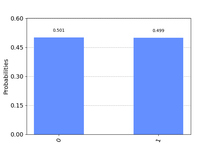
Initializing a Qubit in Superposition
Earlier in this article, we had learned how to initialize a qubit into a given state by using a state vector assignment. Using a state vector, we set a qubit to hold a value of either 0 or 1. However, a qubit can be placed in many different states, including an indeterminate state of both 0 and 1, called superposition.
Let’s see an example of initializing a qubit into superposition with Python Qiskit.
1 | from math import sqrt |
In the above example, we’re initializing the qubit with a state vector of 1/sqrt(2), 1j/sqrt(2). Python uses the “j” to denote a complex number imaginary unit.
If we plot a histogram of the resulting shot values from a qubit in superposition, we can see the resulting values are 0 for 50% of the time and 1 for the other 50% of the time.
We can similarly initialize a superposition state vector for a qubit using an alternative value, as shown below.
1 | state_vector = [sqrt(1-.5), sqrt(1-.5)] # [0.70710678118, 0.70710678118] |
These two state vector assignments work as they are both equal in value to 0.70710678118.
1 | sqrt(1-.5) |
It’s important to note that the sum of the amplitudes-squared for a state vector on a qubit must always equal one. If any values are used where the sum of the squares do not add to one, Qiskit will throw an exception: “Sum of amplitudes-squared does not equal one.”
In the above case of superposition, our state vector values worked since:
1 | 0.70710678118^2 + 0.70710678118^2 = 0.5 + 0.5 = 1 |
Initializing a Qubit to a Variable Degree
Just as we’ve initialized the state vector for a qubit into a superposition of 50/50, we can similarly initialize the qubit to any degree in between.
As an example, let’s initialize the qubit for 1/3 probability of measuring a 0. We can do this with the code below.
1 | qc = QuantumCircuit(1, 1) |
Running the above code will produce the following output.
As we’ve just placed the qubit into a state of having a 1/3 probability of measuring as 0, let’s verify that the same qubit has a 2/3 probability of measuring as 1. We can do this with the code shown below.
1 | # Verify the probability of a 1 is 2/3. |
After executing the above code, we can see the resulting state vector for the qubit is [0.5773502691896257, 0.816496580927726] (corresponding to 0.5773502691896257^2 + 0.816496580927726^2 = 0.333 + 0.6667 = 1. After executing the job, the shot count is {'1': 691, '0': 333} which indicates a 1/3 probability for a 0 and a 2/3 probability for a 1. Likewise, our calculation on the difference between 2/3 and the count divided by total shots, gives us a result of 0.008 which is very close to our exact target of 2/3. If we use an error threshold of +/- 0.03 this is acceptable.
1 | 0.00813802083333337 < 0.03 = True |
Collapsing a Superposition
In the above section, we’ve placed a qubit into superposition and plotted a histogram of its values, proving a 50/50 probability of measuring 0 or 1 (the qubit has a value of both 0 AND 1).
One important rule for superposition is that the moment the qubit is measured, the quantum system collapses into a definite state of 0 or 1. We can prove this by adding a measure statement to our qubit circuit and plotting a histogram of the resulting qubit value.
Let’s start by slightly changing our superposition qubit code to simulate the qubit (without executing on the number of shots).
1 | from math import sqrt |
The above code will output the following state vector for the qubit:
1 | [0.+0.70710678j, 0.70710678+0.j] |
The above values indicate a 50/50 probability for 0/1 with the qubit in superposition. If you run the same program multiple times, you will always see the same values for the qubit state vector.
Now, let’s measure the qubit in superposition, and note how its state collapses into a determinate value of 0 or 1. We will use the measure_all method which concatenates a barrier, classical registers, and measure gate(s) onto the circuit. It’s important to note that if you already have classical registers on the circuit, or if you call measure_all() multiple times, you will be appending multiple classical registers and measure gates onto the same circuit!
1 | from math import sqrt |
You’ll notice in the output from the above code that we will see the output of [0.+1.j 0.+0.j] or [0.+0.j 1.+0.j] about half the time for each. The qubit state vector is collapsing into a value of either 0 or 1, rather than a combination of the two values while in superposition.
Quantum Circuit Identities
Certain quantum gates can be constructed through composition of other gates. Several examples are shown below,
X = HZH
Z = HXH
HSH = HTTH
Additionally, phase gates have identity matches as well. Once a qubit is placed into superposition using the Hadamard (H-gate), the following identities apply:
S = TT (S = pi/2, T = pi/4)
Z = SS (Z = pi)
Z = TTTT
You can confirm the above identities with a Bloch sphere by first using the H-gate and then applying the S, T, Z gates to view the resulting phase change on the qubit.
We can also confirm the Z-axis phase gate identities with the IBM Quantum Composer. Examples are provided for S to TT and Z to SS to TTTT.
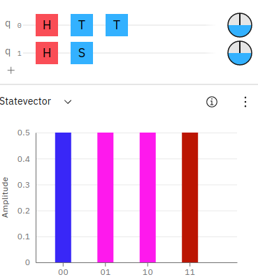
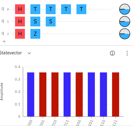
Notice, in the above screenshots the state vector colors match up sequentially for the phases on the qubits. You can also notice the phase disks, along the right side of the circuit layout also match up with equal phases on the qubits.
Creating an X-gate from HZH
An interesting way to create an alternative X-gate (or NOT operator) is to combine an H,Z,H gate. We can prove this in the IBM Quantum Composer as shown in this example.
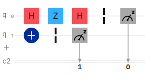
In the above example, the first qubit has an H,Z,H circuit setup to emulate an X-gate. The second qubit has just an X-gate. We can then compare the result for equality.
If we initialize the first qubit q0 to equal 0 and the second qubit to equal 0, the resulting probability will be 11. Likewise, if q0=1 and q1=1, the result will be 00.
Entanglement
So far, we’ve worked with single and multi-qubit quantum computing logic gates that operate largely on well defined states of 0 or 1. However, as we’ve seen above, it’s also possible to place a qubit into superposition. In this section we will see how to place two qubits (i.e., 2 qubits) into superposition in an entangled state.
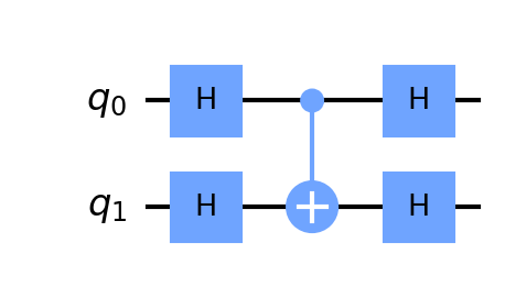
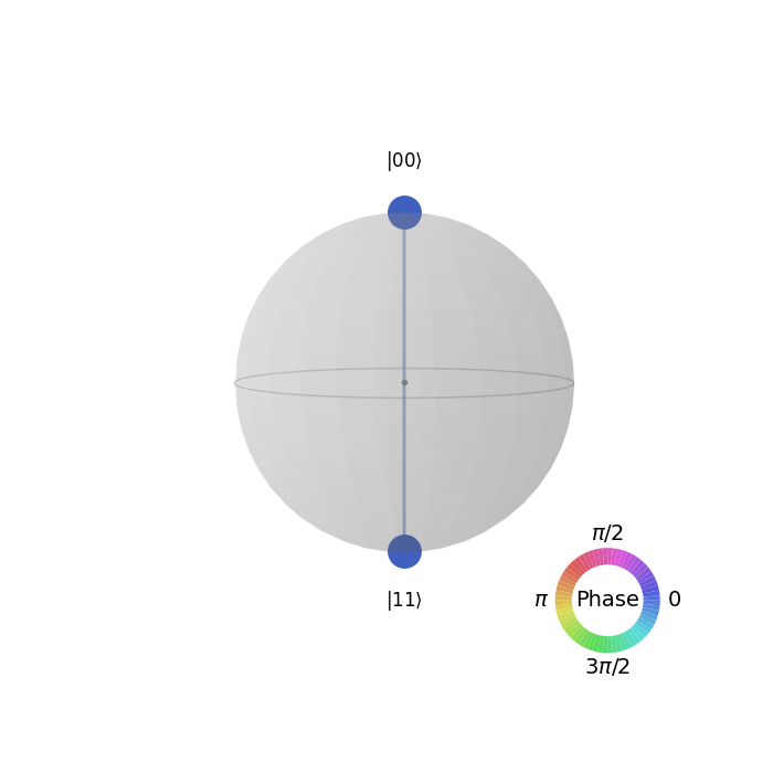
Creating a Bell State in [00, 11]
We can use the h() operator to place a qubit into superposition by using the Hadamard gate. An example of this is shown below.
1 | qc = QuantumCircuit(2, 2) |
The above code executes a Hadamard gate on the first qubit. We then utilize a CNOT gate between the two qubits to effectively entangle them. The resulting output of this circuit appears as shown below.
1 | {'00': 509, '11': 515} |
Likewise, we can view the state vector of the result 2-qubit system, as follows below.
1 | qc = QuantumCircuit(2) |
The above code will produce the following output state vector.
1 | [0.70710678+0.j, 0.+0.j, 0.+0.j, 0.70710678+0.j] |
We can view the probabilities to confirm 00 and 11 having equal chances by plotting a histogram of the results.
Creating a Bell State in [01, 10]
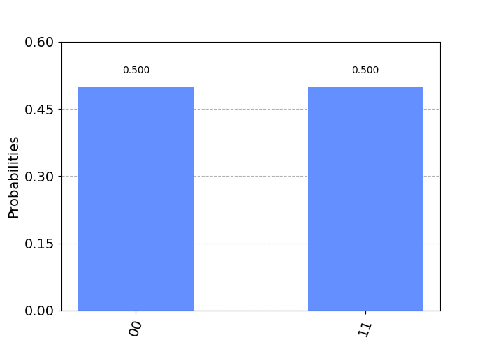
We’ve just seen in the above example, how to implement 2 entangled qubits, also called a Bell State. In the example, our qubits entered an entangled state of 00 and 11. Executing the circuit will always produce a 50/50 chance of seeing 00 or 11, but never 01 nor 10.
In order to change the Bell State to produce the alternate form, we can simply apply an X-gate as shown below.
1 | qc = QuantumCircuit(2, 2) |
The above code produces the following output.
1 | {'10': 489, '01': 535} |
 using the code shown below.
1 | def four_bell_states(): |
The output from the above code is shown below.
1 | [0.70710678+0.j 0. +0.j 0. +0.j 0.70710678+0.j] |
Swapping 2 Bits
In both Qiskit and the IBM Quantum Composer, there exists a quantum swap operator that simply swaps the values of the bits at each position in the input.
An example of swapping bits on a 2-bit string, would produce the following output:
1 | 00 => 00 |
As seen from the source code, we can implement our own swap circuit by using CNOT operators as shown below.
1 | def swap(b, a): |
The above Python Qiskit code sets up a quantum circuit with 2 qubits and 3 CNOT operations in order to swap the input bits and save them to the output.
Demo on IBM Quantum Composer.
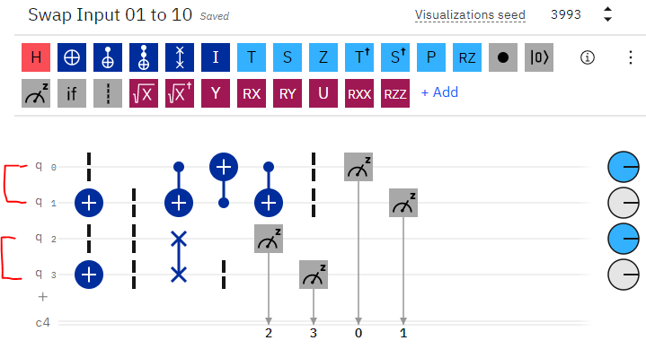
We can confirm the correct behavior of the above circuit by comparing it to the built-in “swap” method, as shown in the screenshot above. Notice, the first 2 qubits are our input, which result in a swapped value for each bit at the far-right output. Additionally, the bottom 2 qubits are an additional input (for testing), where we simply use the built-in swap operator to perform the same operation and confirm the same output result.
We can also confirm the correct result in Qiskit by using a simple test driver code, as shown below.
1 | def swap_test(b, a): |
The above code produces the following output below. Note, the most significant bit is to the left, with the least significant bit on the right, as is standard in bit strings and IBMQ/Qiskit.
1 | 00 => 00 ? True |
If you work through this example, you’ll also notice the circuit has a total depth of 5.
1 | [0 0] |
To preserve the input bits during the swap, we could include an additional two qubits. In this manner, we can see the full swapped bits consisting of input/output. This code is shown below.
1 | def swap(self, b, a): |
The above code produces the following output for all combinations.
1 | {'1001': 1024} |
Notice in the above output, the two right-most bits (least significant) are the input 01 and the left-most bits (most significant) are the output 10.
Swapping n Bits
We’ve just seen how to swap the values of two qubits. Similarly, we can apply the same process to swap any number of bits. We can do this by matching the corresponding qubits with a CNOT to swap their values accordingly.
As an example:
1 | 100000 => 000001 |
Notice how the bit on the left is swapped with its matching bit position on the right. Then we step inward a position and swap the two bits on either end. We repeat the process until we’ve swapped all corresponding bit positions.
As an example, consider 6 qubits. We can swap their values using the following set of CNOT operations.
1 | # Swap the qubits, right-most with left-most. |
Of course, we can generalize the above process for any length bit string by incrementing the index for swapping at each step. The Qiskit code to swap n bits is shown below.
1 | def swap(self, bits): |
If we were to add print statements inside the for loop to view the swapped positions, the following output would result:
1 | swap([1,0,0,0,0,0]) # {'000001': 1024} |
Some additional examples are shown below.
1 | swap([1,0,0,0,0,0]) # {'000001': 1024} |
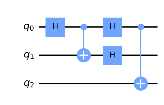
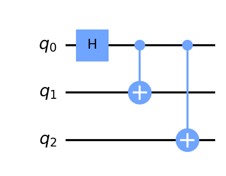
Creating a GHZ State
A Greenberger–Horne–Zeilinger or GHZ is a quantum state is a quantum system that entangles at least 3 qubits.
We can create a GHZ state circuit by using the H and CNOT operators on at least 3 qubits as shown below.
1 | qc = QuantumCircuit(3) |
You can see an example of the GHZ state quantum circuit implemented in IBMQ with a correct output of 50/50 probability for occurrences.
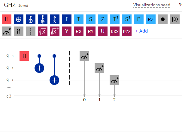
1 | {'000': 481, '111': 519} |
A Unitary Matrix for a Quantum Circuit
So far, we’ve seen examples of creating a quantum circuit using a state vector, in order to initialize the state of the qubits. We’ve also seen how to execute the quantum circuit and obtain the resulting state vector using the ‘statevector_simulator` backend simulator in Qiskit.
While a state vector is the current state for the qubits in a circuit, a unitary matrix is a value for the entire quantum circuit itself.
A unitary matrix can be used to examine the overall processing of a quantum circuit.
To create a unitary matrix, we can use the Qiskit backend unitary_simulator to return a unitary matrix for the circuit.
Let’s create a simple quantum circuit consisting of a single qubit.
1 | qc = QuantumCircuit(1) |
The unitary matrix from the above quantum circuit is shown below,corresponding to our qubit in a state of [01 / 10].
1 | [[0.+0.j 1.+0.j] |
Similarly, as the number of qubits within our circuit expands, so too does the resulting unitary matrix. We can demonstrate this by creating a quantum circuit with two qubits and examining the resulting unitary matrix.
1 | qc = QuantumCircuit(2) |
The resulting unitary matrix for two qubits is shown below. Notice how the size of the matrix has expanded to 4 rows. The unitary matrix increases in complexity according to 2^q where q is the number of qubits. For example, 3 qubits would produce a unitary matrix with 8 rows.
1 | [[0.+0.j 1.+0.j 0.+0.j 0.+0.j] |
Similar to the above examples for producing a unitary matrix by executing quantum gates, we can also initialize a state vector for the qubits in the quantum system and view the resulting unitary matrix.
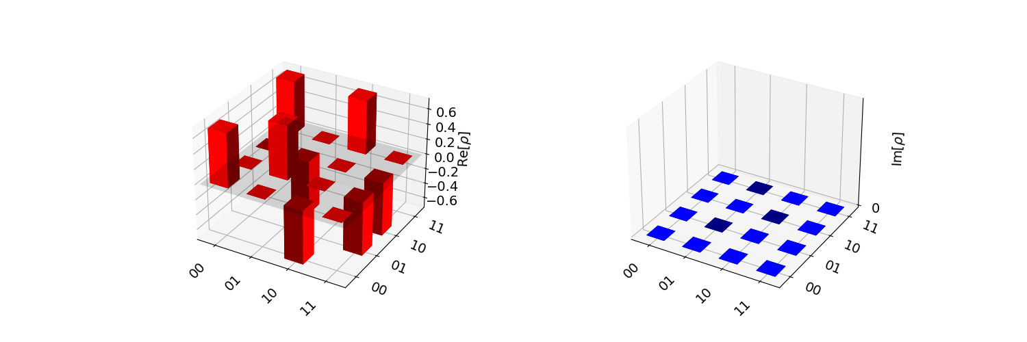
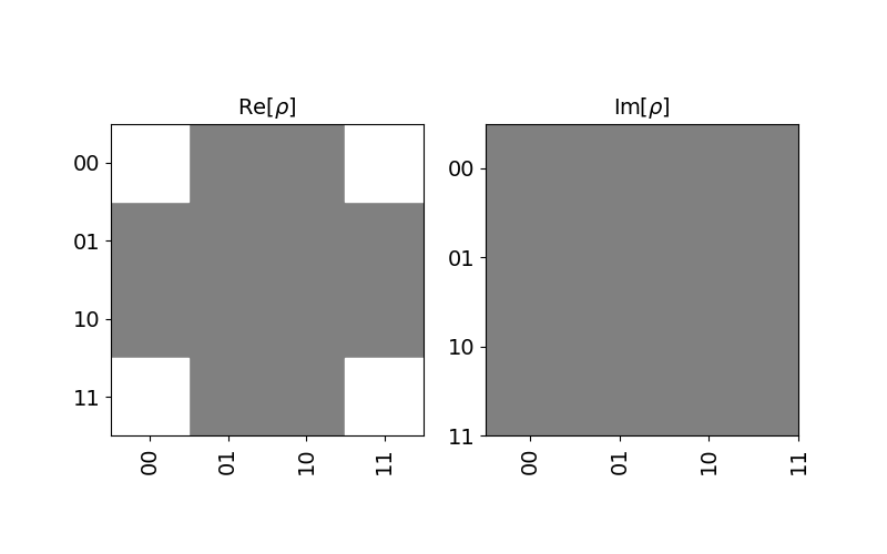
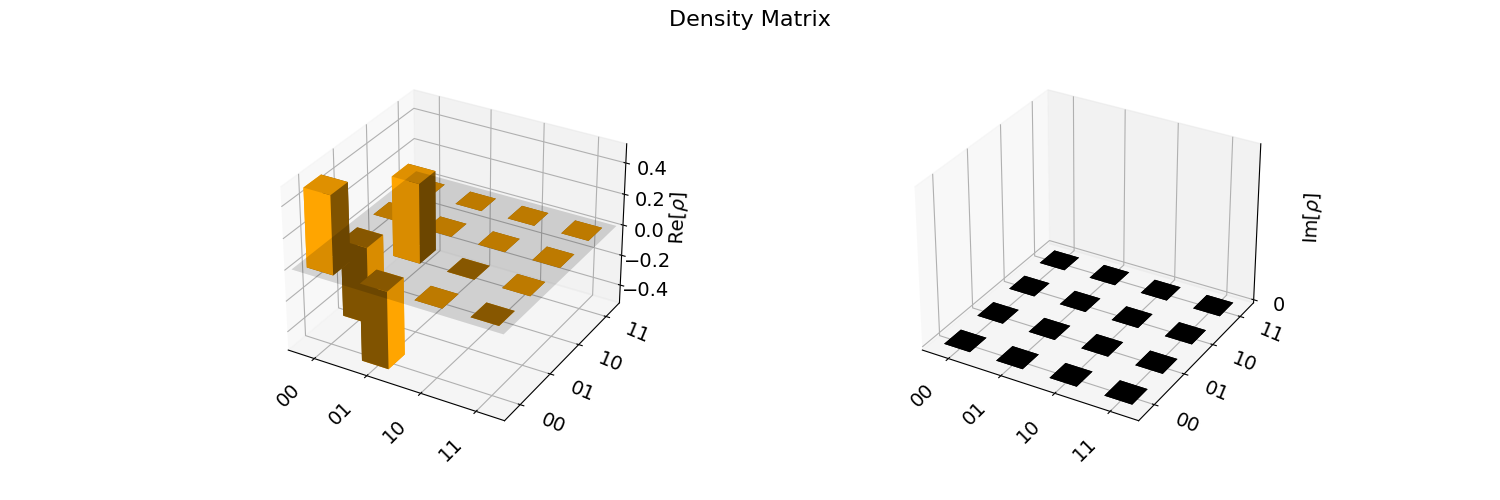
Let’s create a basic Bell state with two entangled qubits and then plot the resulting unitary matrix.
1 | qc = QuantumCircuit(2) |
In the above code, we’ve initialized our two qubits with a superposition state vector. We’ve then used the unitary simulator to obtain the resulting unitary matrix for the qubit states. The output of the resulting Bell state is shown below.
1 | [[ 0.707+0.j 0. +0.j -0.707+0.j 0. +0.j] |
Additionally, we can plot a visualization of the result using plot_state_city as shown below.
Phase Kickback and Reversing a CNOT Gate
As we’ve seen earlier, we can connect a multigate CNOT between two qubits to flip the value of the second qubit when the first one has a state of 1. However, what if we wanted to do the reverse?
Consider the case where we want to use a CNOT between two qubits, but instead of the typical q0->q1 connection where q0 serves as the input control and q1 serves as the output, we want q1 to serve as the input and q0 be the output. How can we turn a CNOT gate upside down?
It turns out that through a process called phase kickback we can take advantage of unique properties of a quantum circuit in superposition in order to allow multigate control operations to behave in reverse.
The key to implementing phase kickback in Qiskit, in order to reverse a multigate control operator, is to enclose the multigate operator within Hadamard gates. That is, both qubits should use double Hadamard gates with the control operator between them.
Let’s see the code for how to reverse a CNOT gate by using phase kickback.
1 | qc = QuantumCircuit(2) |
Notice in the above code, we place both qubits into superposition using the Hadamard gate. We then create a CNOT between qubits 0 and 1, finally closing the circuit with another set of Hadamard gates. We then obtain the unitary matrix for the resulting quantum circuit.
The output from the unitary matrix can be visualized with Latex and saved to an image as shown below.
1 | \begin{bmatrix} |

Just to confirm the correct behavior of the reversed CNOT gate implemented through phase kickback, we create a second quantum circuit. This time, we do not use the Hadamard gates, and instead, just directly connect the second qubit to the first with a reverse CNOT gate (Qiskit allows both directions). We then simulate the unitary matrix and compare it against the first. As expected, both unitaries are equivalent!
1 | Verifying phase kickback CNOT == reverse CNOT: True |
Using the Barrier Operation
The barrier operation creates a visual barrier in a qubit or series of qubits. The barrier operation is primarily a visual effect, to allow easier reading and display of the quantum computing circuit. It is often used to separate sub-circuits within a larger circuit.
However, it is important to note that a barrier also indicates to the Qiskit transpiler to not simplify the circuit in the separating barriers. This can be useful, for example, to measure effects from noise introduced by gates.
In Qiskit, the barrier operation can be applied to all qubits, an array of qubits by index, or a specific qubit by index. Also, since the barrier operation does not actually perform any changes, it is not included when calculating the depth of a circuit.
An example of using the barrier operation is shown below.
1 | qc = QuantumCircuit(2) |
The output of the above barrier operations is shown below.
1 | # Barrier all qubits. |
Note, the barrier operation can accept no arguments, in which case it places a barrier across all qubits, or a comma-separated list, or an array of indices to place a barrier upon the qubits.
The following code places a barrier across the first and last qubits.
1 | qc = QuantumCircuit(3) |
Retrieving the Qiskit Version
It may be necessary to determine the specific version of Qiskit running on a machine. Getting the Qiskit version, backend provider version, and other specific version details can be done in the following ways, as shown below.
First, let’s retrieve a simple version number for Qiskit.
1 | from qiskit import qiskit |
1 | 0.18.0 |
Next, let’s retrieve the detailed version information for Qiskit.
1 | qiskit.__qiskit_version__ |
1 | {'qiskit-terra': '0.18.0', 'qiskit-aer': '0.8.2', 'qiskit-ignis': '0.6.0', 'qiskit-ibmq-provider': '0.15.0', 'qiskit-aqua': '0.9.4', 'qiskit': '0.28.0', 'qiskit-nature': None, 'qiskit-finance': None, 'qiskit-optimization': None, 'qiskit-machine-learning': None} |
If you’re running on a Jupyter notebook, there are a variety of other Jupyter-specific tools that can be called for version information.
1 | import qiskit.tools.jupyter |
While qiskit.__version__ and qiskit.__qiskit_version__ both seem similar, the web site indicates that the version, alone, can be misleading as it returns only the version for the qiskit-terra package. Therefore, it is recommended to use the full qiskit_version value.
See the topic Checking Which Version is Installed for more details.
Running on a Real Quantum Computer with IBMQ
So far, we’ve executed quantum circuits on Qiskit simulators. However, you can also run quantum computing circuits on quantum computers hosted by IBMQ. Calls are executed via the IBMQ API over the Internet. You’ll need to sign-up in order to obtain an API key to access your account and execute code on the remote servers.
The following examples show how to run a quantum circuit on an IBMQ quantum computer. The first step is to load your IBMQ account using your API key.
1 | from qiskit import IBMQ |
Once your account has been loaded, you can retrieve a backend provider to execute code on a quantum computer.
1 | # Retrieve a list of providers. |
The list of backends for IBMQ is shown below.
1 | [<IBMQSimulator('ibmq_qasm_simulator') from IBMQ(hub='ibm-q', group='open', project='main')>, <IBMQBackend('ibmqx2') from IBMQ(hub='ibm-q', group='open', project='main')>, <IBMQBackend('ibmq_armonk') from IBMQ(hub='ibm-q', group='open', project='main')>, <IBMQBackend('ibmq_santiago') from IBMQ(hub='ibm-q', group='open', project='main')>, <IBMQBackend('ibmq_bogota') from IBMQ(hub='ibm-q', group='open', project='main')>, <IBMQBackend('ibmq_lima') from IBMQ(hub='ibm-q', group='open', project='main')>, <IBMQBackend('ibmq_belem') from IBMQ(hub='ibm-q', group='open', project='main')>, <IBMQBackend('ibmq_quito') from IBMQ(hub='ibm-q', group='open', project='main')>, <IBMQSimulator('simulator_statevector') from IBMQ(hub='ibm-q', group='open', project='main')>, <IBMQSimulator('simulator_mps') from IBMQ(hub='ibm-q', group='open', project='main')>, <IBMQSimulator('simulator_extended_stabilizer') from IBMQ(hub='ibm-q', group='open', project='main')>, <IBMQSimulator('simulator_stabilizer') from IBMQ(hub='ibm-q', group='open', project='main')>, <IBMQBackend('ibmq_manila') from IBMQ(hub='ibm-q', group='open', project='main')>] |
You can filter the list of backends to select a specific one, as shown below.
1 | # Filter by actual quantum computers that are operational. |
Finally, let’s run a quantum circuit for a Bell state on the quantum computer.
1 | qc = QuantumCircuit(2, 2) |
The output from running our Bell state on a quantum computer is shown below.
1 | {'00': 363, '01': 129, '10': 166, '11': 366} |
Notice the counts for the results are highest at 00 and 11 which is the expected output from our Bell state. The remaining counts are due to error rates on the physical quantum computer.
Monitoring the Status of a Job
We can monitor the run status of a job on a quantum computer or on the simulator by using several commands as shown below. As an example, let’s run the same Bell state circuit from the prior section on a simulator and compare the resulting counts.
1 | from qiskit.tools import job_monitor |
The output from the simulator is as shown below. Notice, we’ve used the job_monitor and job.status methods to obtain information about the running job.
1 | {'11': 495, '00': 529} |
As expected, the results from the Bell state are a 50/50 split (with a far smaller rate of error than an actual IBMQ quantum computer) of 00 and 11.
Visualizing Quantum Circuits
A variety of methods are available for visualizing quantum circuits, qubits, and vectors. These vary depending on the type of graphical output and the type of input. For example, quantum circuits can be drawn in ASCII text, graphically as a png, or even as latex output. Qubits can be drawn in 3-dimensional spheres, called qspheres, Bloch spheres, and phase disks. Result counts from qubit measurements can be viewed using text, histograms, and state vectors.
Let’s take a look at how to generate some of the different visualizations of quantum circuits and qubits using the Qiskit visualization tools.
Visualizing a State Vector
We’ll begin with viewing a state vector for a Bell state. We should be getting fairly familiar with creating these simple circuits. The code for our Bell state is shown below.
1 | from qiskit.quantum_info import Statevector |
The above code calls the draw method on the Statevector object and returns an IPython Latex object for display within a Jupyter notebook. To access the raw latex data, we can view figure.data which returns $$\n\n\\begin{bmatrix}\n\\tfrac{1}{\\sqrt{2}} & 0 & 0 & \\tfrac{1}{\\sqrt{2}} \\\\\n \\end{bmatrix}\n$$.
It may be simpler to draw the state vector in text. We can call state_vector_ev.draw('text') which results in [0.70710678+0.j,0. +0.j,0. +0.j,0.70710678+0.j].
We can draw the state vector in other formats as well.
1 | figure = state_vector_ev.draw('qsphere') |
The above code results in the following plots.
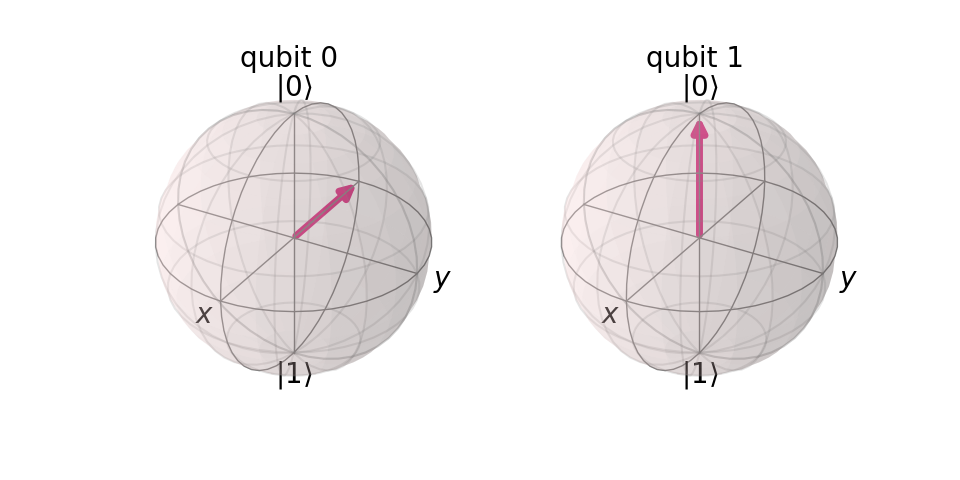
Displaying plot_bloch_vector versus plot_bloch_multivector
The two methods for displaying a Bloch vector include plot_bloch_vector, which requires specific coordinates to manually display a Bloch sphere using either cartesian or spherical coordinates, and plot_bloch_multivector which takes a Statevector (such as from a QuantumCircuit) and displays the associated qubits.
1 | figure4 = plot_bloch_vector([0,0.25,1]) |
Displaying Quantum Circuits
Let’s take a look at how to draw quantum circuits with some of the more advanced visualization features. We’ll start with a basic GHZ gate.
1 | ghz = QuantumCircuit(3) |
The Difference between a Bloch sphere and a Q-sphere
In the section above, we’ve demonstrated some of the visualization techniques for quantum computing systems, including the Bloch sphere and the Q-sphere. It’s important to note the difference between these two visualizations, as they are distinctly different, even when used to display a single qubit.
The Bloch sphere is intended for the view of a single qubit. It provides visual information similar to a phase disk or result count histogram. The Bloch sphere is a localized view of the current, with each qubit viewed separately.
The Q-sphere, by contrast, is a global view of a quantum system. It displays visual information about the entire quantum state of the system, which includes the full global environment.
Between the two visualizations, a Bloch sphere is useful for displaying information about a single qubit. A Q-sphere is useful for displaying information about multiple qubits together in an overall system.
Exporting QASM
QASM is a quantum computing programming language, more formally called OpenQASM. It’s a quantum computing language specific to building quantum circuits. It allows the design of universal quantum computing using models and measurements.
The OpenQASM specification has more details on the language and how to use it. Below is an example of creating a basic quantum circuit using OpenQASM.
1 | // Initialize and flip a qubit, then measure the result. |
We can export QASM directly from a Qiskit quantum computing circuit by using the qasm() method, as shown below.
1 | qc = QuantumCircuit(2, 2) |
The result of the above QASM export is shown below.
1 | 'OPENQASM 2.0; |
Additionally, we can import a QASM string or file into a Qiskit circuit to rebuild a quantum computing design, as shown below.
1 | # Load from a QASM string. |
Plotting Gate Maps and Error Rates
In addition to the Qiskit quantum computing visualizations that we’ve already seen, including the histogram, Bloch vectors, Q-spheres, and State vector plots (Hinton, state city density, etc), we can also view plots of physical quantum backend providers, such as IBMQ.
Specifically, we can plot a gate map and error map for a physical quantum computing device.
A gate map shows the connections between nodes on a physical quantum computing device.
An error map shows both the node connections of a gate map, in addition to the error rate expected on the backend.
Before we can plot device data, we’ll need to connect to an instance of IBMQ. The code below demonstrates how to connect to an instance of IBMQ using your API account, retrieving a backend provider, and plotting the gate map and error map for the backend.
1 | from qiskit import IBMQ |
The above code produces the following two charts from the provider’s backend on IBMQ.
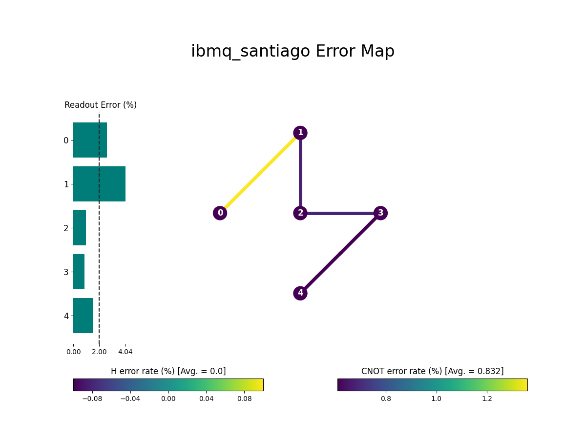
Notice how the gate map is actually a subset of the overall error map plot, which shows additional information, including the error rates associated between device nodes.
One additional note on connecting to IBMQ, if you’re network requires a proxy connection due to a firewall, you can use the following code to connect to IBMQ via a proxy.
1 | proxies = {'urls': { 'http': 'http://your.proxy.com:80', 'https': 'https://your.proxy.com:80'}} |
Creating Phase on Qubits
We’ve seen several examples of using quantum computing operators to change the probability outcomes for measured qubits on the X and Y axis. These include the Hadamard, X, CX, RX, RY, and other gates, all of which alter the X/Y axis and the resulting qubit probability. While these gates allow changing the probabilities for outcomes, they do not change the qubit phase on the Z-axis, which remains at 0. To change the phase and the resulting phase disk (which provides the local state of each qubit at the completion of a quantum computing computation), we use a different set of quantum computing gates.
Changing the phase variance for a qubit can be done by using the gates S, T, Z, and P. Respectively, these change the phase on a qubit by pi/2, pi/4, pi, and a custom value (such as pi/8).
In fact, the Z gate is similar to the “X” gate, in that it flips the value of the Z-axis from 0 to 1 or from 1 to 0 (i.e., a full inversion of pi). The remaining gates alter the Z-axis by a predefined amount in reference to pi.
Let’s take a look at some quick examples of modifying the phase for a qubit. We can do this within the IBM Quantum Composer.
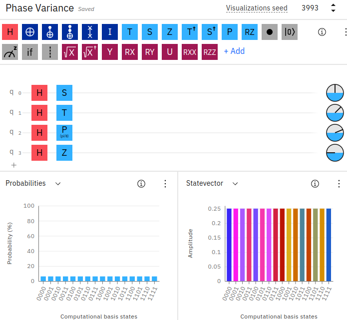
In the above example on IBM Quantum Composer, we’ve created 4 qubits and placed each one in superposition using the Hadamard gate. We’ve then applied a Z-axis modifier to each qubit. The first qubit is using the S-gate, and as a result of applying it to the qubit, the phase becomes pi/2. Similarly, the second qubit using the T-gate has a phase of pi/4, followed by a P-gate with a custom theta value set of 8 resulting in pi/8 (you can right-click the gate to change the custom theta value), and finally the Z-gate with a full inversion of the Z-axis of pi.
You can also see the small circle phase disks located towards the right of each qubit line, indicating the amount of phase variance that each qubit is resulting in. Additionally, notice in the state vector chart there is an array of colored outcomes due to the varying phases for the results, while the probability outcomes remain evenly split across all qubits (as we’re only using the Hadamard gate, which results in a 50/50 outcome - hence an event split across all possibilities).
The corresponding Qiskit code for implementing the phase on the qubits in this example can be found below.
1 | from qiskit import QuantumRegister, ClassicalRegister, QuantumCircuit |
Keep in mind, similar to the section above on “Quantum Circuit Identities”, the S, T, and Z-gates are equivalent to each other according to the number of applications for pi. For example, S = TT (since S = pi/2, T = pi/4) and Z = SS (since Z = pi and two S-gates equal pi/2 + pi/2 = pi). Likewise, Z = TTTT (since T = pi/4 and four T-gates equal pi/4 * 4 = pi).
Plotting Phase in a Q-Sphere
We were able to view the colorful state vector plot in IBM Quantum Composer for the phases of our qubits. You can perform a similar visualization in Qiskit by plotting a Q-sphere for the quantum circuit, which displays a global view of the entire quantum circuit and its included qubits together in a single visualization, as shown below.
1 | from qiskit import qiskit, QuantumRegister, ClassicalRegister, QuantumCircuit, BasicAer, execute |
In the above code, we’re using 3 qubits in superposition, and then applying the S, T, and Z gates to each one. This alters the phase for each qubit on the Z-axis. We can then display the result (similarly, colorful!) in a Q-sphere. Notice, we can simply call the draw method to plot the qsphere, as it is built-in to the Statevector object.
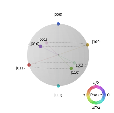
The qsphere above can be plotted in Qiskit using the above code or an alternate version which executes the quantum circuit and retrieves the state vector after simulation.
1 | backend = BasicAer.get_backend('statevector_simulator') |
The above code will plot the same result as the q-sphere shown above. The difference is that we’ve executed the circuit and retrieved a state vector. In this case, we need to call the actual plot_state_qsphere(sv_ev2) method and pass in the resulting state vector to display.
Quantum Fidelity
Quantum fidelity allows you to obtain a measurement of the amount of distance between two quantum gates, states, or processes.
A formal definition states that quantum fidelity is a measure of how “close” two quantum states are, in that one state will effectively identify as another.
As a rule of thumb, fidelity is simply measuring the amount of “noise” that you can expect between your code and actual physical quantum hardware.
Since quantum measurements typically involve noisy environments and are prone to specific rates of error, fidelity is a means of measuring just how close you can expect your quantum circuit programming code to execute compared to when running on physical quantum computing hardware, after taking into account expected noise and error rates. This is especially the case with “gate” fidelity, which measures the error on a quantum gate (such as x, s, t, z, y, etc) compared to an actual gate operation on a quantum computer.
When a measurement for quantum fidelity is a value of 1, this refers to two states that are equivalent. Similarly, when considering only global phase between two operators using the same gate calculations, the result is an average gate fidelity and process fidelity of 1, since both average gate and process fidelities deal with global phase, compared to state fidelity which measures a single state vector.
Qiskit offers several methods for measuring fidelity, as available in qiskit.quantum_info.state_fidelity.
State fidelity measures between two quantum states (such as statevectors or density matrix objects).
Process fidelity measures the noise within a quantum channel or operator.
Average gate fidelity measures the fidelity of multiple gates within a quantum channel. Note, average gate fidelity requires the channel and target operator to have the same dimensions and input/output dimensions.
Measuring State Fidelity
Here is a quick example of measuring state fidelity for two quantum circuits.
1 | from qiskit.quantum_info import state_fidelity |
The output from the above program will print 1.0 as the resulting state fidelity. This means that both quantum circuits are equivalent. By contrast, let’s try measuring two different quantum circuits.
1 | qc1 = QuantumCircuit(2) |
In the above example, the first quantum circuit places both qubits into superposition. However, the second only places one qubit. The result is a state fidelity of 0.5.
Measuring Average Gate and Process Fidelity
Next, let’s see an example of measuring the average gate fidelity between two custom operators.
1 | from qiskit.quantum_info.operators import Operator |
In the above code, both the average gate fidelity and process fidelity are 1.0. By contrast, let’s create two distinctly different operators and measure the average gate fidelity.
1 | from qiskit.quantum_info.operators import Operator |
As expected, the above code using two different operators (S and Z) produces an average gate fidelity of 0.667 and a process fidelity of 0.5.
Quantum Fidelity with Identities
Earlier we took a look at quantum computing identities, such as an S-gate being equivalent to two T-gates, or a Z-gate being equivalent to two S-gates. We can confirm these identities by using fidelity measurements. Some examples are shown below.
S to TT
1 | qc1 = QuantumCircuit(1) |
The output from the above identity is 0.99, nearly a perfect equivalency.
Z to SS
1 | qc3 = QuantumCircuit(1) |
The output from the above identity is 0.99.
Just for comparison, let’s see the fidelity for a non-equivalent circuit. We’ll just compare two of the prior circuits and check their fidelity measurement.
1 | print(average_gate_fidelity(qc1, qc3)) |
This time, the average gate fidelity output is 0.66 and the process fidelity is 0.49, as the circuits are not equivalent.
Density Matrices
Density matrices are often useful in initializing quantum circuits. Qiskit provides the DensityMatrix object for easily working with these data structures. Below is an example of combining two density matrix objects into a single matrix using the tensor method.
1 | from qiskit.quantum_info import DensityMatrix |
The result of the above tensor command will output the following DensityMatrix.
1 | DensityMatrix([[0.5 +0.j, 1. +0.j, 0.25+0.j, 0.5 +0.j], |
Creating Custom Gates
Quantum circuits can be packaged into custom gates that may be re-used within new quantum circuits. This can be done by using the to_gate method, as shown below.
1 | # Start by creating a quantum circuit, in this case, a Bell state. |
The above code results in the following new circuit using a custom gate.
1 | q_0: ────────────── |
Notice how the custom gate spans across qubits q_1 and q_2 (qubits 2 and 3 in our circuit). The custom gate takes 2 inputs and 2 outputs, since our original quantum circuit used 2 qubits.
Composing Circuits from Other Circuits
You may have noticed the append() operation in the preceding section, which allows you to append a gate onto an existing quantum circuit. Similar to this, we can also use the “compose” method or plus operator to build a quantum circuit using existing quantum circuits.
An example of composing a quantum circuit from an existing one is shown below.
1 | qc1 = QuantumCircuit(2, 2) |
In the above code, we’ve created two separate quantum circuits. We join them together by using the “compose” method. This creates a new quantum circuit consisting of the bit-flip operator followed by the measurement gates.
We can also use the “add” method to perform the same effect, although with slightly less flexibility.
1 | qc3 = qc1 + qc2 |
It’s also important to note that you can combine quantum circuits together inline and perform operations. For example:
1 | (qc1+qc2).draw() |
Decomposing a Quantum Circuit
We can decompose a quantum circuit to see the contents of its gates. This is often useful in the case of custom gates, in order to view the contents within. Using the example of our custom gate from the above section, we can decompose it as shown below.
1 | qc2.decompose().draw() |
1 | q_0: ─────────────── |
Notice how we’ve decomposed the custom gate back into its original quantum circuit, except it’s now placed across q_1 and q_2 as we indicated in our append command.
Enhancing Gates with Additional Controls
Quantum gates typically take a certain number of input qubits and target qubits as output. For example, an X-Gate takes a single qubit as both input and output, while a CX-Gate takes one control qubit as input and one target qubit for output.
We can further modify gates to take additional qubits as input, in which case they behave similarly to a CX-Gate, or rather, a “controlled” N-gate.
Below is an example of adding an additional control to a Y-gate, making it a controlled Y-gate that will only perform the Y operation if the control qubit has a value of 1.
1 | from qiskit.circuit.library import YGate |
This results in the following circuit, notice the control qubit set to q_0 and the target on q_1.
1 | q_0: ──■── |
Multiple controls can be added to a gate in either direction, qubits at the front or at the end, with respect to where the gate is positioned. For example, the following code adds our custom_gate (created earlier in the section above) with two control inputs and two target qubits in either direction.
1 | qc_multi = QuantumCircuit(4) |
The above code results in the following circuit below.
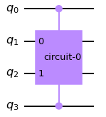
Notice how the above code places a control at qubit q0 and another control on the last qubit q3, with the custom_gate sitting in the middle across qubits q1 and q2. In the “append” method, we specify [0, 3, 1, 2] as the position arguments, which correspond to 0, 3 as the control inputs and 1, 2 as the target.
Passing Arguments to Controlled Gates
In addition to specifying the control qubits and target qubits, some gates require additional arguments such as theta values. In these cases, the arguments are usually provided before the control indices.
Below is an example of creating a controlled RZ gate and passing a value for theta.
1 | qc = QuantumCircuit(3) |
Notice in the above code, we first provide the value for theta, followed by the control qubit index (1) and the target qubit (2).
About the Author
This article was written by Kory Becker, software developer and architect, skilled in a range of technologies, including web application development, artificial intelligence, machine learning, and data science.
References
Preparing for the Qiskit Developer Certification Exam
IBM Qiskit Developer Certification Exam PDF Topic List
Bartu Bisgin’s Jupyter Notebook Study Guide
Ved Dharkar’s Jupyter Notebook Collection
IBM Certified Associate Developer - Quantum Computation using Qiskit v0.2X
Fundamentals of Quantum Computation Using Qiskit v0.2X Developer - C1000-112 - IBM Quantum
Sponsor Me