Introduction
Can we program a quantum computer to output the text “Hello World”? As it turns out, it’s entirely possible. In fact, we can utilize one of the principal quantum computing algorithms, Grover’s Search, in order to not only create a quantum computing program that can output “Hello World”, but to also demonstrate a quadratic reduction in time complexity for executing the software!
In this article, we’ll create a quantum computing program that can output the phrase “Hello World” to the screen (in addition to any text or phrase that you’d like!). Our solution will use the Grover’s Search algorithm in order to locate the target letters that make up the phrase. We’ll provide a random array of letters as input to our quantum computing program and allow the quantum computing algorithm using Grovers Search to locate the target letters from the array and assemble them accordingly to complete our phrase. Finally, we’ll output the result!
Why Hello World?
In software programming, the Hello World program is intended to be a simple and understandable introduction to a new programming language or paradigm. It’s often used for students to understand a new programming language and try their first attempts at creating a program in that language.
Writing a program to output “Hello World” targets a couple of key tasks in any computer programming solution. These include assembling a string of ASCII characters, accessing the print or output command, and of course, structuring a start and end of the program. Ultimately, it also demonstrates a complete working computer program solution.
Shifting Over to Hello World on a Quantum Computer
Naturally speaking, writing a Hello World program for a quantum computer may not seem like the most feasible task for a quantum computing program to solve.
Quantum computers are (currently) primarily used for mathematical and logical calculations, taking input as numeric values and output numeric values in return. The results of quantum computing programs are often used within other mathematical calculations. Quantum computers are rarely (if ever?) used to perform a trivial activity such as outputting text to the screen!
However, the goal of this article is not to answer the question “should we do it”, rather it’s to demonstrate that “yes, indeed, we can do it”!
More realistically, by developing a Hello World quantum computing program, we’ll demonstrate a key feature behind quantum computing solutions, by realizing a quadratic time complexity reduction in execution time over a typical searching algorithm on a classical computer, in addition to demonstrating how to implement Grover’s Search algorithm on a quantum computer using Qiskit and Python.
Now that you’re convinced and excited about the potential of a Hello World program running on a quantum computer, let’s move on to the details about why we’ll use Grover’s Algorithm.
Searching for a Needle in a Haystack
Before we dive into the solution, it’s important to first understand the reason behind using Grover’s Search algorithm.
Suppose that we have a random array of items (we’ll be using ASCII letters in this case [‘c’, ‘a’, ‘b’, ‘d’, etc.]. However, the random items could be anything.). If we wanted to locate the index of a specific item from the list of random items, we obviously would need to walk through the entire list, from beginning to end, until we find the value that we’re looking for. This makes perfect sense. If the value is located at the front of the list, we’ll find it on the first look. If the value is located at the end of the list, we’ll have to walk through the entire list before we find it.
On a classical computer, searching through an unsorted list of values will take O(n) time complexity. This means that in the worst case scenario, where our target value is at the end of the list, we need to look through the entire list to the end, until we find the value.
The Advantage of Using a Quantum Computer
A quantum computer can utilize Grover’s algorithm to find the target element within the array of unsorted values in O(sqrt(n)) time complexity. This is a quadratic speed-up in time complexity, compared to a classical computer!
A quantum computer achieves this dramatic reduction in processing time by representing each bit in the length of the array with a qubit. For example, an array of 8 random items can be represented on a quantum computer using just 3 qubits. This provides 2^3=8 possible combinations, enough to represent each potential index in our array of random items. Since a quantum computer can calculate all possible values for qubits within a quantum circuit in a single cycle, the program can evaluate all potential indices in the array during a single CPU cycle in the process of searching for the target element.
It’s important to note that in this article we are simplifying some of the ideas behind Grover’s Search algorithm in order to make it easy to understand. However, this process serves to demonstrate the difference in CPU processing time between a classical computer and a quantum computer in searching and locating the desired elements (which in this case, will be ASCII letters that make up our target phrase, “Hello World”).
The Method Behind Our Madness
Let’s take a look at exactly how we’ll design our quantum computing program using Qiskit and Python to output “Hello World”.
We’ll start by simplifying our goal to just output the word “hello”. Therefore, consider that we have the following array of randomly generated letters that we want to search through to produce the word “hello”.
1 | ['a','y','h','p','e','o','l','l'] |
Our goal will be to go letter by letter, check if the letter exists in the array, and if it does, find the index for it. We’ll store these indices and finally output the letters at each index to the screen, resulting in our final output of “hello”.
That is, our algorithm will function as follows:
- Generate an array of random letters.
- Find the index of each letter in our target string from within the array. *
- Store the indices found.
- Output the letter located at each index to the screen.
Step #2 is the most complex part of the process. In fact, this is the key part of our demonstration of the difference between a classical and quantum computer.
We’ll be using classical computing commands with Python to generate the array of random letters, store the indices in a variable, and print the result. However, searching through the array is where the true CPU processing takes place.
Running on a Classical Computer
On a classical computer, given the above random array of letters, if we wanted to produce the word “hello” by selecting the index for each letter, we would need to search across the array for each item.
For the first letter, ‘h’, we search up to index 3 and locate the letter. For the second letter, ‘e’, we search up to index 5 and locate the letter. However, for the third letter, ‘l’, we need to search through the entire array, all the way to the end, in order to locate the letter at index 7.
In the worst-case scenario, this algorithm on a classical computer requires searching through all elements and therefore has a time complexity of O(n).
Even worse, for the entire phrase “hello”, this would be a time complexity of O(n*m), where n = length of the array of letters (8) and m = length of the word “hello” (5).
Now, we can optimize on this process by leveraging a hashmap to store the indices of the elements on our first pass through the array of random letters. This would take O(n) to create the hashmap of the indices, since we still need to traverse the entire array. However, we could then iterate through each letter in our target string to retrieve the index from the hashmap, instead of having to go back through the array again. This would still take O(m), where m = length of the word “hello” (5), since each look-up in the hash is a single execution of O(1), plus the cost to build the hash in the first place, of O(n).
The optimized version can reduce the total time complexity from O(n*m) to O(n+m) => O(n).
Keep in mind, the time complexity may seem trivial when dealing with just 8 random elements in an array. However, what if our array consisted of 8 million elements instead? Or perhaps, even 8 trillion? This is where a quadratic speed-up in time complexity could provide an incredible difference in processing time - and a quantum computer does just that!
The Speed Up on a Quantum Computer
Now that we’ve seen how a classical computer can solve our algorithm, let’s see how a quantum computer can boost the time complexity with a quadratic reduction in time searching through the array of unsorted values.
On a classical computer, a single bit can only represent one of two values - 0 or 1. This is how an electronic transistor works. It’s either open or closed. It’s either zero or one.
By contrast, a quantum computer uses qubits. A single qubit on a quantum computer can represent two values virtually simultaneously (at the time of computation). A qubit can be in the state of 0 and 1 during a single quantum computing CPU cycle.
Therefore, a classical computer can represent information in bits by processing n bits per CPU cycle.
1 | 1 bit = 0, 1 (2 CPU cycles to process all states) |
However, a quantum computer can process these states simultaneously, and therefore can process 2^n qubits per CPU cycle.
1 | 1 qubit = 0, 1 (1 CPU cycle to process) |
It’s this exponential difference in processing power that makes a quantum computer so powerful! Just to extrapolate this idea, a quantum computer with only 50 qubits can process 2^50=1e+15 bits of information during a single cycle, compared to a classical computer that can simply process 50 bits of information with the same number of transistors.
Running our Algorithm on a Quantum Computer
Let’s walk through how our program will leverage the above speed-up in processing time on a quantum computer.
As we’ve seen above, we can represent information using qubits, which allow us to leverage 2^q states per CPU cycle, where q = number of qubits.
We can represent each index within the array of random letters using enough qubits to represent the length of the array. In our example, we have an array of length 8. Thus, we can represent this number of indices in the array using 3 qubits, since 2^3=8 possibilities for 3 qubits.
Imagine the 3 qubits in this example, 000, 001, 010, 011, 100, 101, 110, 111 being searched simultaneously for the target letter. During a single CPU cycle on a quantum computer we can look in the array at each possible index and determine if the target letter is located at this slot. After just 1 cycle, we can return the index 011=3 for the letter ‘h’. Likewise, in a single cycle, we can locate the letter ‘l’ at the last index of 111=7.
This solution has a time complexity of O(sqrt(n)). For the entire phrase “hello”, we iterate across each letter in the target phrase, totalling 5 times to search, and execute the quantum circuit each time. Just as with our classical computing algorithm, this would take an additional O(m), where m = length of the phrase “hello” (5).
This is a total time complexity of O(sqrt(n)+m) => O(sqrt(n)).
The Great and All Knowing Oracle
Now that we’ve compared a classical implementation to a quantum implementation of our Hello World algorithm, let’s see how to actually build this for a quantum computer.
As we’ve discussed earlier, we’ll be using the Grover search algorithm to implement our program on a quantum computer. This particular algorithm, like many quantum algorithms, requires an oracle.
An oracle is a black-box mechanism for indicating to the quantum program circuit when a correct solution to a problem has been found. The oracle is encoded directly into the quantum circuit at the time of programming it, and executed as part of the entire quantum program. The quantum circuit essentially checks against the oracle at each iteration in order to move closer towards the correct solution for qubit values. Without an oracle, the quantum computing algorithm would be unable to determine when it has located the correct letter in the sequence for our target phrase in the “Hello World” program.
In a nutshell, the oracle tells our quantum program when the configuration of qubit values (0’s and 1’s) corresponds to the letter ‘h’, or the letter ‘e’, or any of the letter ‘l’ elements in our target phrase. Of course, we will need to update the oracle for each letter, since the index for each letter is different.
Creating the Oracle
Now, an oracle can be created in a variety of ways. For example, an oracle can consist of logic that determines a solution state, given the values of the qubits being evaluated, or it can simply give the solution state (which is the method we will be using in this article).
For example, consider a game of simplified Sudoku. In this game, we have a 4x4 board where a unique number must exist in any row or column, with no duplicates. We could design an oracle using logical constraints for this problem by representing clauses for the qubits. Since each configuration of qubit values can represent different combinations of clauses, we can determine when a satisfactory solution is found for those clauses. That is, when the clauses represent a state where no duplicate value exists in any row or column. In this case, that set of clauses (i.e., the configuration of qubit values) becomes the solution to the quantum circuit.
The above link gives a great example of building this type of oracle. However, for the sake of keeping this article simple and easy to understand, we’ll be creating a static type of oracle that simply “knows” the index of the target element that we’re searching for. This oracle will guide our quantum circuit towards arriving at the correct configuration of qubits for our answer.
Let’s take a look at a concrete example of creating a static type of oracle. That is, an oracle that encodes the answer within its circuit (rather than using logical clauses and constraints, this oracle simply encodes to desired qubit configuration).
The most common way to create a static oracle for Grover’s algorithm is with the Z-Gate.
Using the Z-Gate in an Oracle
One of the easiest ways to create an oracle for Grover’s search algorithm on a quantum computer is to utilize a controlled Z-Gate. The Z-Gate will allow us to flip the phase of a single amplitude of the quantum circuit. This sets the detection for Grover’s algorithm to identify the target answer.
The way this is done is to apply a controlled Z-Gate across each qubit in the circuit. It does not matter which qubit serves as the target versus the control(s) for the Z-Gate, as long as all qubits are included in the controlled Z-Gate process.
For example, suppose we want our algorithm to find the state 1111. We can use the following oracle as shown below.
1 | q_0: ──■───── |
If we want any of the qubits to have a value of 0, we can simply insert an X-Gate (NOT gate) into our circuit on both sides of the desired qubit. Since HXH=Z and HZH=X, we can take advantage of the quantum identities to create a multi-controlled phase circuit from a series of X-gates.
An example of finding the state 1011 is shown in the following Qiskit code.
1 | # Create a quantum circuit with one additional qubit for output. |
The above code results in the following oracle.
1 | q_0: ──────■────── |
Notice how we’ve applied an X-Gate around the Z-Gate control for qubit 2 (note, we count qubits from right-to-left using Qiskit standard format).
The output from running Grover’s algorithm with the above oracle is shown below.
1 | {'1101': 48, '0001': 47, '1100': 52, '0101': 40, '0100': 49, '0110': 46, '1110': 56, '0010': 63, '1000': 61, '1011': 264, '1111': 46, '1010': 54, '1001': 51, '0000': 49, '0111': 58, '0011': 40} |
Notice that the number of occurrences for our target value 1011 has the highest count of 264. This indicates the solution to our problem!
Let’s take a look at another example of creating a simple oracle with the controlled Z-Gate.
Finding all Odd Numbers
Suppose that we want to find all odd numbers within a specific range of qubits. For example, from 3 qubits we can create 2^3=8 possible values, including the values 0 through 7. This is shown below in binary form from each qubit.
3 qubits
1 | 000 = 0 |
We can see how each of the odd numbers contain a 1 for their rightmost digit (in binary). Therefore, we can create an oracle for Grover’s algorithm to find all measurements of qubits that result in a 1 for the rightmost digit. This is done by applying a controlled Z-Gate from the rightmost qubit to all other qubits. That is, we want only the rightmost qubit to be the “control”, while the other qubits serve as the “target” to apply the phase flip to.
The oracle to find odd numbers can be created in Qiskit with the following code.
1 | qc = QuantumCircuit(4) |
Alternatively, we can use the following shortcut syntax.
1 | n = 4 |
This results in the following oracle.
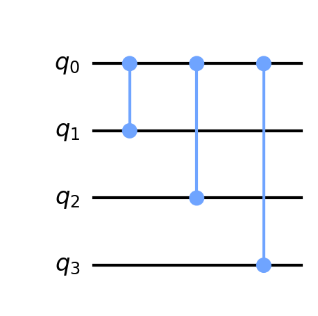
1 | q_0: ─■──■──■─ |
Notice, we’ve used a controlled Z-Gate from qubit 0 (the rightmost qubit in Qiskit standard format) and attached this gate to each of the other qubits as targets. When qubit 0 has a value of 1, the Z-Gate is applied to all of the other qubits, setting the matching phase for Grover’s algorithm.
Output
The result of running Grover’s algorithm with the odd numbers oracle is shown below.
1 | {'111': 254, '001': 232, '101': 275, '011': 263} |
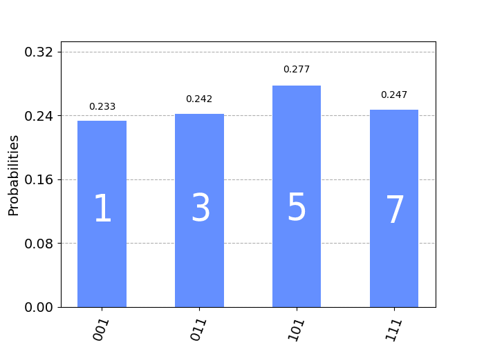
The above result shows how the measurements are spread equally across each of the odd numbers within the range of 3 qubits. Notice how each measurement found has the rightmost bit set to a value of 1.
Of course, we don’t have to stop at just 3 qubits. Let’s see the result from 5 qubits.
1 | {'01101': 68, '01001': 48, '10101': 69, '10111': 47, '00001': 77, '00101': 71, '01011': 68, '10011': 56, '01111': 65, '10001': 72, '11011': 71, '00111': 55, '00011': 66, '11101': 63, '11001': 61, '11111': 67} |
Again, we can see how the measurements from the resulting quantum computing program are split evenly across all odd numbers in the range of 5 binary digits (5 qubits).
Finding all Even Numbers
Just to hammer in the idea of using the controlled Z-Gate to create a static oracle, let’s find all even numbers within a range of qubit values.
With the odd number oracle we simply applied a Z-Gate from qubit 0 to all other qubits. This had the effect of flipping the phase of the other qubits when qubit 0 had a value of 1. However, this time we want to do the opposite! We only want to flip the phase of the other qubits when qubit 0 has a value of 0. Do you think you know how to achieve this now?
We simply surround the target qubit with X-Gates, of course! This has the effect of flipping the qubit before applying the controlled Z-Gate. Note, we will also need to “unflip” the first qubit back to its original state, in order to preserve the circuit for Grover’s algorithm. This oracle is shown below.
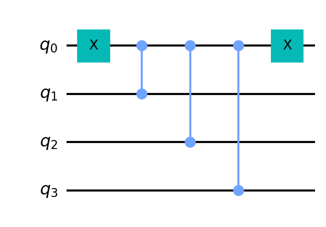
1 | ┌───┐ ┌───┐ |
The above oracle for measuring even numbers is nearly identical to that for measuring odd numbers. The only difference is the additional X-Gate applied to the first qubit, ensuring that we only flip the other qubit phases when qubit 0 has a value of 0.
Output
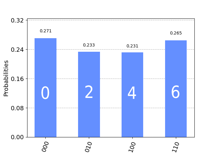
The result of measuring for even numbers for 3 qubits is shown below.
1 | {'100': 242, '000': 271, '010': 260, '110': 251} |
Creating Logic Clauses for an Oracle
We’ve just demonstrated how to encode an oracle on a quantum computer for running Grover’s algorithm to find target value(s) from a configuration of qubits. In these examples, we’ve seen how to encode a specific target value (such as 1011) and how to encode a range of values (such as odd or even numbers).
Now, what if we’re not sure of the target value ahead of time. Even more important, what if we want to find multiple values!
Is there a way to create the oracle in a more automatic fashion, inserting the appropriate gates on the circuit without us having to determine which qubit should receive the X-Gate(s) and which qubit should be the control versus target for the controlled Z-Gate(s)?
As it turns out, Qiskit provides an extremely convenient helper method for automatically generating logical circuits. We can use this to build the appropriate series of controlled X-Gates to target specific qubit configurations.
The way that we do this is to create a logical function for the correct qubit values and provide this function to the oracle. We are going to use this technique to specify the correct index to our target letters in our “Hello World” algorithm!
To create a logical function, we first identify the value that we’re looking for. For example, suppose we want a quantum circuit to find the values 0 and 3. 011.
We formulate a logical clause using the following Python function structure.
1 | (not x1 and not x2 and not x3) or (x1 and x2 and not x3) |
We pass this clause into our oracle builder, which returns a QuantumCircuit object. We will be leveraging the Qiskit methods ClassicalFunction and synth in order to automatically generate the quantum circuit from the Python function.
1 | # Convert the logic to a quantum circuit. |
This generates the following quantum circuit for the above example.
1 | (not x1 and not x2 and not x3) or (x1 and x2 and not x3) |
We can then insert this quantum circuit directly into our parent quantum circuit program to complete Grover’s algorithm.
Keep in mind, typically an Oracle does not know ahead-of-time what the correct solution is, rather it formulates the solution from given clauses and identifies the qubit solution values. However, for this example, we are more or less directly providing the Oracle with the solution via a logical function (to serve as our clause) in order to demonstrate a simple example of searching for elements in an unordered list.
Mapping Qubits to Letters
You’re probably getting an idea at this point that we can utilize the logical oracle technique to identify the indices within our array of random letters to guide the quantum circuit into finding the correct letter. If so, you’re exactly right! Now, we just need to figure out how to map the qubits to the letters within our array.
Let’s consider an array of random generated letters that we want to search through to form the word “hello”.
1 | ['a','y','h','p','e','o','l','l'] |
The length of this array is 8 and we can represent this using 3 qubits, since 2^3=8. This means we can get 8 different combinations of values from those qubits, corresponding to all possible indices in our array.
When our quantum program runs, the circuit will simultaneously evaluate all possible combinations of qubits, calling the oracle against each combination, and getting back an indication (via the phase-flip) of which combination of qubit values is a valid solution.
For the letter ‘h’, the only solution is at index 2 or 010.
1 | Index of 'h' = 2 |
For the letter ‘l’, we have two solutions at index 6 (110) and 7 (111). The oracle would return a “high” result for both indices in the solution so that after our quantum circuit runs for the letter ‘l’, we would get the following result below.
1 | Index of 'l' = [6,7] |
For each letter in the target phrase, we configure the oracle as we’ve described above (using the logical clause technique for our oracle) and execute the quantum circuit for one iteration. We then measure the outcomes from each possible combination of qubit values. The maximum measurement count result will be our target index for the letter.
For the case of ‘h’, we would expect to see low measurement counts for all 3-bit combinations of qubit values except for the state 010, which corresponds to index 2 in our array of random letters, i.e., the letter ‘h’.
We repeat this process for each letter in the target string.
For the word “hello”, we will run the quantum circuit 5 times. On a classical computer, this would require 5*8=40 iterations, with 8 indices in the array to search across, multiplied by 5 letters in the target phrase. If we use the hash optimization technique described earlier in this article, we can reduce the time down to 8+5*1 iterations (8 iterations to move across the array and store the letters in the hash plus 5 cycles to lookup each letter within the hash, with each lookup taking a constant time of 1). However, on a quantum computer this would only require 5*1=5 CPU cycles, including a single iteration for initialization and executing the quantum circuit for each letter in our target word or phrase.
That’s it! This is the technique that we’ll use to create our “Hello World” example and demonstrate it executing on a quantum computer.
Since we’ll need to generate random letters, the following code below will generate a random array of letters for a specific size in Python.
1 | def random_letters(n): |
Executing the above code can generate a random array of letters as shown below.
How Many Qubits Do We Need?
There may be one more question in your mind before we jump into the results. We can come up with any target phrase that we want our quantum circuit to generate. However, how do we figure out how many qubits to use in our circuit? Let’s consider the number of possible values that can be represented from a specific number of qubits.
If we have 1 qubit, we can have 2 possible values: 0 or 1
If we have 2 qubits, we can have 4 possible values: 00, 01, 10, 11
If we have q qubits, we can have 2^q possible values: 001, 010, 011, 100, 101, 110, 111, etc.
Now, consider the target word “hello” which consists of 5 letters. Additionally, consider that we will use an array of 8 random letters (including each letter in the phrase that we want to find combined with the random letters). We know that we can represent 8 possibilities using 3 qubits, since the maximum binary value from 3 qubits would be 111=7. This corresponds to the values 0-7 (or 8 total possibilities). Each possibility maps to an index in the array.
Using the above knowledge, we can calculate the required number of qubits. Since our target phrase is 5 letters, we can calculate the logarithm of 5 in base 2 (for binary). Thus, log(5, 2)=2.3. Since we can’t have a fraction of qubits in a quantum circuit, we simply round up and take the ceiling value of this result. This allows us to determine the number of qubits needed for any length of word or phrase!
Calculating the Number of Qubits from Letters
The following examples show the number of qubits needed for differing lengths of letters.
For 5 letters, ceil(log(5, 2)) = 3 qubits (111 = 0 to 7 = 8 possible values)
For 9 letters, ceil(log(9, 2)) = 4 qubits
For 15 letters, ceil(log(16, 2)) = 4 qubits (1111 = 0 to 15 = 16 possible values)
For 16 letters, ceil(log(17, 2)) = 5 qubits (11111 = 0 to 31 = 32 possible values)
For 33 letters, ceil(log(33, 2)) = 6 qubits (111111 = 0 to 63 = 64 possible values)
etc.
Grover’s Search Quantum Circuit
We’ve now discussed how to create an oracle to implement Grover’s search algorithm in a quantum computing circuit with Python and Qiskit. Next, let’s see the actual implementation of Grover’s search in Python and Qiskit.
Grover’s search is a quantum computing algorithm that utilizes amplitude amplification in order to identify solutions. When the algorithm finds a subset of qubit values that match the oracle (for example, 110 or 010), the amplitudes for those qubits are increased, resulting in a higher measurement, thus marking the solutions.
Grover’s search algorithm requires two parts. The first part is the iteration step of the algorithm. This step initializes the quantum circuit and executes the black-box oracle. This iterative step may be required to execute several times before filtering out the correct solution, depending on how many qubits are part of the quantum computing circuit. For our example, typically one iteration is sufficient.
The second step involves diffusing the circuit. This amplifies the inputs of correct solutions, allowing those combinations of qubit values to gain momentum in measurements, resulting in the answer. This is performed via the oracle so that correct combinations of qubit values result in the highest amplitudes.
In order to focus on the oracle design for our Hello World program, the mathematical principles behind the Grover algorithm and amplitude amplification can be reviewed further. There is a fantastic article on implementing Quantum Pokemon Fight with Grover’s search.
Let’s view a brief overview of the steps below.
- Initialize the quantum circuit to the superposition state.
- Perform the Grover iteration step(s).
- Measure the resulting quantum circuit to obtain the answer.
Let’s take a look at the Python code to implement the algorithm.
Grover’s Search Iteration
The code below implements the Grover’s search algorithm iteration.
1 | from qiskit import QuantumCircuit |
Notice, in the above code we begin by initializing a QuantumCircuit in Qiskit. We then flip the value of the qubits from 0 to 1 in order to designate a phase-flip for our circuit (which is how our oracle will mark correct solutions). We then place the qubits in superposition via qc.h(n). Following, we execute the oracle. Finally, we execute the diffuser process. The last step is to undo the phase-flip by placing all qubits back from superposition and flipping the qubits again from 1 to 0.
Grover’s Search Diffuser
The code below implements the Grover’s search algorithm diffuser.
1 | def diffuser(n): |
Executing the Quantum Circuit
With the algorithm defined, we can execute the complete quantum computing circuit in Python with Qiskit on both the simulator and real-device at IBMQ. The code to execute the circuit is shown below.
1 | import ast |
The above code allows us to pass in a QuantumCircuit object to be executed, which in our case will be the QuantumCircuit object returned from our method grover(). The code also supports using a configuration file to designate running on a simulator or on a real quantum computer at IBMQ by specifying an API key. It also supports the use of a proxy (if you are running from behind a corporate firewall, for example) through the configuration file.
1 | [IBM] |
Our “Hello World” Quantum Circuit
With the above code, we can now visualize the complete Grover’s Search algorithm quantum computing circuit in Python and Qiskit. The circuit is shown below.
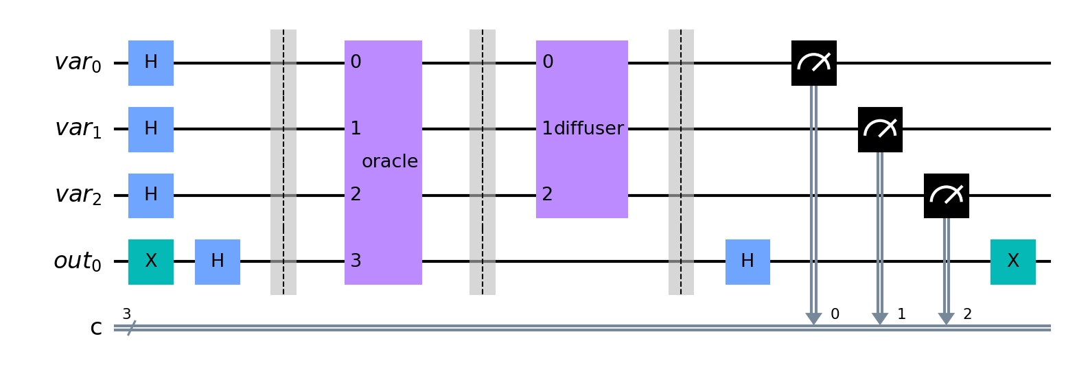
Notice the initialization steps at the beginning (left-most) part of the circuit. This places the qubits into superposition and flips the values to indicate a phase-flip. In between the barriers is our black box gate for the oracle, which spans across all qubits on the circuit. The gate covers all qubits in order to apply the appropriate phase-flip to indicate the solution. Next, we apply the diffuser for amplitude amplification across the input qubits. Finally, we again execute the superposition step and undo the flip of the qubit values, with a measurement across all input qubit values to indicate the result.
Our implementation is now complete. Let’s put it all together and see the result!
Putting It All Together
With our Python Qiskit functions defined for creating the quantum computing circuit, we can put this all together for our “Hello World” program. An excerpt of the code is shown below.
1 | phrase = 'hello' |
After our quantum computing circuit runs, we will have a resulting array of indices containing the location of each letter from our array. We can now just walk through the indices to output the result!
1 | for i in range(len(indices)): |
Results
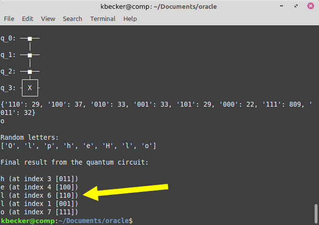
Below is the output from running the program for the word “hello”. Notice, we print out the logical-clause oracle circuit used in searching for each letter.
1 | 3 qubits, 8 possibilities |
Single Letter H
In the output from the program above, we’re displaying the oracle used when searching for each letter. Remember, a unique oracle is created for each search, and inserted into the Grover search algorithm quantum computing circuit.
Let’s focus in on one of the letters and its associated oracle to see how the measurement results work.
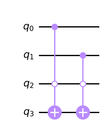
To highlight how the logical-clause oracle is generated, a decomposed view of an oracle for finding the letter ‘h’ in an array of random letters is shown below.
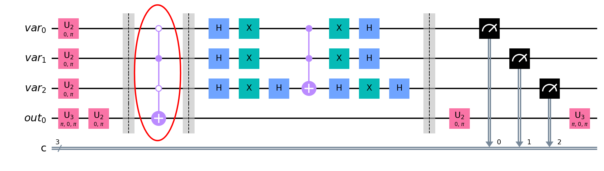
This oracle results in the following measurements.
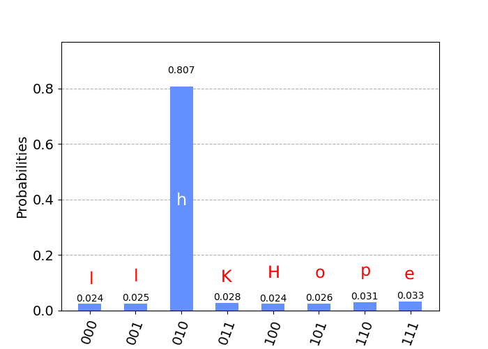
Notice how the value 010 or index 2 has the highest measurement result after executing Grover’s algorithm. This indicates that the letter ‘h’ was present at (zero-based) index 2 in the array.
What if our logical clause is a bit more complex than a single X or Z-Gate. Will Python Qiskit generate a corresponding circuit? Indeed, an oracle can be generated with multiple steps, as shown below.
Notice how we can generate logical-clause oracles that consist of multiple controlled X and/or controlled Z-Gates. This is done automatically for us by the Qiskit Python function, as described above, for generating logical circuits.
Multiple Letters L
Our oracle can clearly identify a single high measurement for the index of a target letter in our array. Now, what if we have multiple occurrences of the target letter?
Our oracle can handle multiple indices and return high measurement counts for these as well!
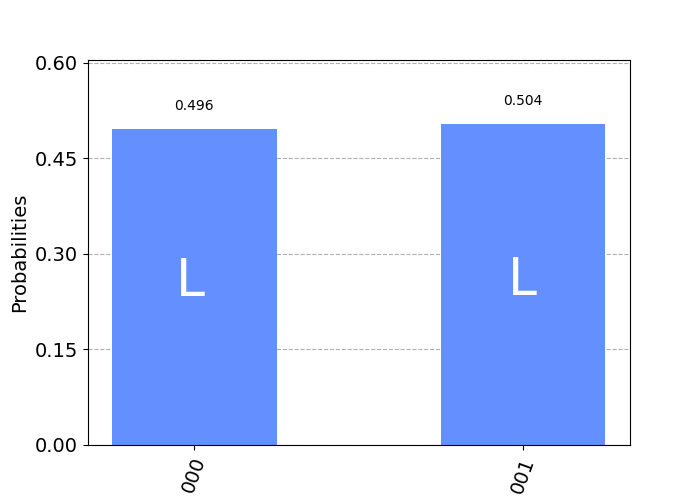
In this example, the letter ‘l’ exists at index 0 and index 1 within our array of random letters. Therefore, the oracle returns high measurement counts for two indices, allowing us to (arbitrarily) choose either index to use in the result.
Power It Up With Longer Sentences and Lots of Qubits
Does this really work for even longer sentences with lots of qubits? It sure does!
1 | 5 qubits, 32 possibilities |
There are quite a few letter ‘l’ elements in the target phrase (and the random array of letters). What does the oracle look like for finding all locations of this letter?
1 | Finding letter 'l' |
What do the measurement results look like for this letter?
1 | {'01100': 1, '00001': 1, '01101': 1, '01110': 2, '11101': 1, '10100': 5, '00110': 2, '01111': 3, '11001': 154, '10001': 1, '01010': 151, '01011': 164, '00000': 171, '00010': 161, '10010': 2, '10110': 2, '10101': 2, '10000': 2, '11100': 171, '11110': 1, '01001': 3, '00101': 2, '10111': 2, '11000': 3, '01000': 4, '11011': 4, '00011': 6, '00100': 2} |
Sure enough, there are 6 high measurement counts, corresponding to the locations of each target index for the letter ‘l’ within the array of random letters!
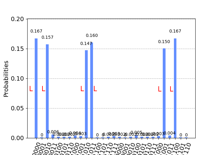
We can clearly see all 6 locations for the letter ‘l’.
Download @ GitHub
The source code for this project is available on GitHub.
About the Author
This article was written by Kory Becker, software developer and architect, skilled in a range of technologies, including web application development, artificial intelligence, machine learning, and data science.
Sponsor Me