Introduction
Determining a person’s gender as male or female, based upon a sample of their voice seems to initially be an easy task. Often, the human ear can easily detect the difference between a male or female voice within the first few spoken words. However, designing a computer program to do this turns out to be a bit trickier.
This article describes the design of a computer program to model acoustic analysis of voices and speech for determining gender. The model is constructed using 3,168 recorded samples of male and female voices, speech, and utterances. The samples are processed using acoustic analysis and then applied to an artificial intelligence/machine learning algorithm to learn gender-specific traits. The resulting program achieves 89% accuracy on the test set.
Update: By narrowing the frequency range analyzed to 0hz-280hz (human vocal range), the best accuracy is boosted to 100%/99%. ∗
Demo
The web-based demo application allows you to upload a .WAV file of a voice. You can alternatively enter a url of a voice recording from vocaroo.com or clyp.it.
Please note, this is a research project! It should not be used as a definitive guide on gender recognition. If a classification seems incorrect to you, it probably is! The models have been trained on publicly available voice datasets that are only a very small range of real-world voices. The demo should be considered for research and entertainment value only.
The Dataset
The complete dataset can be downloaded in CSV format.
In order to analyze gender by voice and speech, a training database was required. A database was built using thousands of samples of male and female voices, each labeled by their gender of male or female. Voice samples were collected from the following resources:
- The Harvard-Haskins Database of Regularly-Timed Speech
- Telecommunications & Signal Processing Laboratory (TSP) Speech Database at McGill University
- VoxForge Speech Corpus
- Festvox CMU_ARCTIC Speech Database at Carnegie Mellon University
Each voice sample is stored as a .WAV file, which is then pre-processed for acoustic analysis using the specan function from the WarbleR R package. Specan measures 22 acoustic parameters on acoustic signals for which the start and end times are provided.
The output from the pre-processed WAV files were saved into a CSV file, containing 3168 rows and 21 columns (20 columns for each feature and one label column for the classification of male or female). You can download the pre-processed dataset in CSV format, using the link above.
Acoustic Properties Measured
The following acoustic properties of each voice are measured:
- duration: length of signal
- meanfreq: mean frequency (in kHz)
- sd: standard deviation of frequency
- median: median frequency (in kHz)
- Q25: first quantile (in kHz)
- Q75: third quantile (in kHz)
- IQR: interquantile range (in kHz)
- skew: skewness (see note in specprop description)
- kurt: kurtosis (see note in specprop description)
- sp.ent: spectral entropy
- sfm: spectral flatness
- mode: mode frequency
- centroid: frequency centroid (see specprop)
- peakf: peak frequency (frequency with highest energy)
- meanfun: average of fundamental frequency measured across acoustic signal
- minfun: minimum fundamental frequency measured across acoustic signal
- maxfun: maximum fundamental frequency measured across acoustic signal
- meandom: average of dominant frequency measured across acoustic signal
- mindom: minimum of dominant frequency measured across acoustic signal
- maxdom: maximum of dominant frequency measured across acoustic signal
- dfrange: range of dominant frequency measured across acoustic signal
- modindx: modulation index. Calculated as the accumulated absolute difference between adjacent measurements of fundamental frequencies divided by the frequency range
Note, the features for duration and peak frequency (peakf) were removed from training. Duration refers to the length of the recording, which for training, is cut off at 20 seconds. Peakf was omitted from calculation due to time and CPU constraints in calculating the value. In this case, all records will have the same value for duration (20) and peak frequency (0).
A Baseline Algorithm for Detecting Voice Gender
In order to determine whether a computer program is actually achieving better results than a non-artificial intelligence based approach, a baseline model can be employed and used to measure initial accuracy.
The first baseline model is a simple algorithm to determine the gender of a voice. It simply always responds with “male” for a voice, regardless of the acoustic properties.
This algorithm results in an accuracy of 50% on both the training and test sets. This makes sense since the dataset is split evenly between male and female voice samples. This is the same accuracy as flipping a coin and guessing randomly. Smarter algorithms can certainly do better than this.
A (Not-So) Simple Threshold on Frequency
Given the measured acoustic properties of a voice, an alternate baseline algorithm can be created by using the frequency of a voice for determining the gender.
At first glance, a simple algorithm of setting a threshold for frequency sounds like a reasonable way to detect gender from voice or speech. Perhaps, a frequency of 200 hz could be used as a dividing line. However, frequency can vary widely within a spoken word, let alone an entire sentence. Frequency rises and falls with intonation, often to communicate certain emotion within words and speech. This can make it difficult to pinpoint an exact frequency.
This hypothesis can be tested by applying a logistic regression model, using the average dominant frequency measured across each voice sample. We can then record how accurately this describes the gender of a voice. Here is an example of building this baseline model in R:
1 | genderLog <- glm(label ~ meandom, data=train, family='binomial') |
The summary output for this model, appears as follows:
1 | glm(formula = label ~ meandom, family = "binomial", data = train) |
We can see in the above summary that the average dominant frequency (meandom) is, indeed, statistically significant with regard to gender. In fact, since the meandom value is positive, this supports our hypothesis that an increase in frequency corresponds with a voice classification of female. Let’s see how well this model performs.
The frequency-based baseline model results in an accuracy of 61% on the training set and 59% on the test set. This is better than the first baseline algorithm, but still far from accurate detection of male/female voices.
This suggests there is more to detecting a voice’s gender than simply applying a threshold on how low or high a voice sounds.
Digging Deeper into Voice Acoustic Properties
Let’s take a look at a full logistic regression analysis of all measured acoustic properties of a voice. This will give us a view of which properties are statistically significant for determining gender. We can build this model in R, as follows:
1 | genderLog <- glm(label ~ ., data=train, family='binomial') |
The summary output for this model, appears as follows:
1 | glm(formula = label ~ ., family = "binomial", data = train) |
There are 15 properties of statistical significance in this model. This suggests that we can benefit by including more properties in our machine learning model to detect gender from speech.
The logistic regression model achieves an accuracy of 72% on the training set and 71% on the testing set. This is clearly an improvement over the baseline algorithms.
Building a CART Model of Voice Acoustics
When utilizing an algorithm such as logistic regression, it can be difficult to determine which exact properties indicate a target gender of male or female. We could guess that it likely one of the statistically significant features, but ultimately this decision breakdown is masked within the model.
To gain an understanding of a trained model, we can apply a classification and regression tree model (CART) to our dataset to determine how these properties might correspond to a gender classification of male or female.
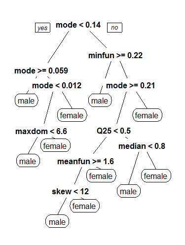
We can see in the above CART tree that the mode frequency (mode) serves as a root node for detecting the gender as male or female. From there, it then checks the minimum fundamental frequency, followed by more specific properties, such as maximum dominant frequency, first quantile hertz, skewness, median frequency, and a further breakdown of mode frequency.
The CART model achieves an accuracy of 81% on the training set and 78% on the test set. This is certainly a positive boost in accuracy.
Random Forest
Similar to the CART classification tree model, we can apply a random forest model. This achieves an accuracy of 100% on the training set and 87% on the test set, which is a further improvement over the CART model.
Boosted Tree
Taking the random forest model a step further, we can apply a generalized boosted regression model, using the gbm package with caret.
The boosted tree model achieves an accuracy of 91% on the training set and 84% on the test set. This is not quite as a good as the tuned random forest, however fine-tuning parameters could be utilized to boost performance.
SVM
Our next model is a support vector machine, tuned with the best values for cost and gamma. To determine the best fit for an SVM model, the model was initially run with default parameters. A plot of the SVM error rate is then printed, with the darkest shades of blue indicating the best (ie., lowest) error rates. This is the best place to choose a cost and gamma value. You can fine-tune the SVM by narrowing in on the darkest blue range and performing further tuning. This essentially focuses in on the section, yielding a finer value for cost and gamma, and thus, a lower error rate and higher accuracy. The following performance images show how this progresses.
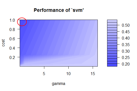
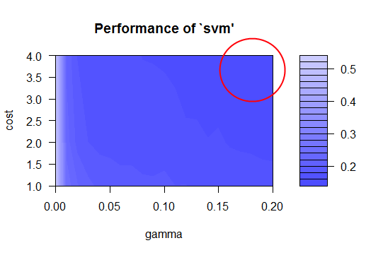
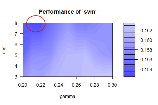
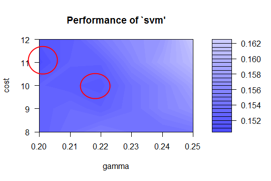
The code for producing the above plots is shown below. Notice how the accuracy increases after each fine-tuning of the cost and gamma properties for the SVM. We also maintain a constant random seed.
1 | set.seed(777) |
Our best SVM achieves an accuracy of 96% on the training set and 85% on the test set. Although this is just slightly less accuracy than the random forest model, we’ll still be able to use the SVM in a stacked ensemble model, which is described below.
XGBoost
We can apply a final model, using the XGBoost algorithm. This model achieves an accuracy of 100% on the training set and 87% on the test set. This results in the highest accuracy of our models, so far.
Stacked Ensemble Model
Up until now, we’ve seen the accuracies from single models applied to the dataset. The best accuracy that we’ve achieved on the test set is 87% with a tuned Random Forest or XGBoost model. An additional technique for boosting accuracy is to combine models together, into a stacked ensemble.
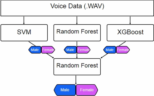
We’ll stack together 3 models: SVM, Random Forest, and XGBoost. Remember, each model outputs a classification of male or female, based upon the audio file. Since each model reports slightly different results, we can take the 3 outputs and feed them into another classification model. This final model can then figure out which of the 3 models to weigh higher, and hopefully increase the accuracy a bit more.
Here’s a diagram of what our ensemble looks like.
The code for creating a stacked ensemble can be found below.
1 | results1 <- predict(genderSvm, newdata=test) |
The stacked model, indeed, performs better. It achieves a 2% increase over the prior best model, reaching a test set accuracy of 89%.
What Exactly is the Model Detecting?
We’ve seen in the above models how the accuracy of classifying male or female voices was increased by including all available acoustic properties of the voices and speech. Determining a male or female voice does, indeed, utilize more than a simple measurement of average frequency. To demonstrate this, several new voice samples were applied to the model, each using different intonation. For example, the first voice sample used flat or dropping frequency at the end of sentences. A second sample used a rising frequency at the end of sentences. When combined with voice frequency and pitch (ie., male vs female voice range), this difference in lowering or rising of the voice at the end of a sentence would occasionally signify the difference in a classification of male or female. This is especially true when the male and female voice samples were within a similar, androgynous, frequency range.
The above described type of classification makes sense, as male and female speakers will often use changing intonations to express parts of speech. Female voices tend to rise and fall more dramatically than their male counterparts, which might account for this difference.
A larger dataset of voice samples from both male and female subjects could help minimize incorrect classifications from intonation.
A Disclaimer on Real World Accuracy
We’ve seen the stacked ensemble model achieve an accuracy of 89% on the test set. This is a positive achievement, although it’s certainly not 100%.
It’s important to keep in mind what the model is actually trained upon. Training data can skew a model from the real world, since the real world often has a much larger variety of data. In the case of voices, there is a large array of both male and female voices that lie within different androgynous zones of frequency and pitch. A dataset that includes a much larger number of samples from the general population would likely train a model that could achieve more accurate results in the wild.
After all, a model is only as good as its data.
Update: Narrowing Acoustics to Within Human Vocal Range
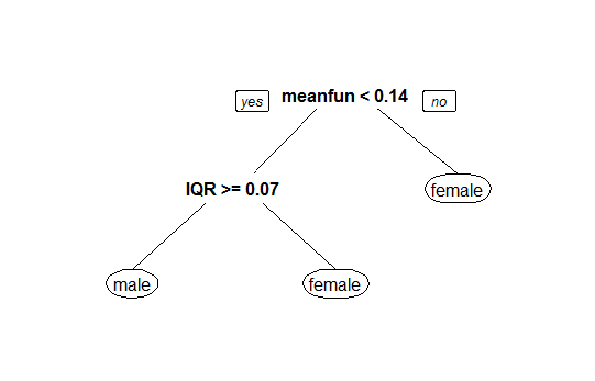
After narrowing the analyzed frequency range to 0hz-280hz (human vocal range) with a sound threshold of 15%, the accuracy is boosted to near perfect, with the best model achieving 100%/99% accuracy.
You can see in the CART model below how “mean fundamental frequency” serves as a powerful indicator of voice gender, with a threshold of 140hz separating male and female classifications.
Download @ GitHub
The source code for this project is available on GitHub.
About the Author
This article was written by Kory Becker, software developer and architect, skilled in a range of technologies, including web application development, machine learning, artificial intelligence, and data science.
Sponsor Me