Revolutionizing the Deutsch-Jozsa Algorithm: A Quantum Upgrade

Introduction

How do you enhance one of the most popular quantum computing algorithms for beginners in order to make it even easier to use and understand? In this article, we’ll see how to enhance the traditional Deutsch-Jozsa quantum computing algorithm to fix several shortcomings, making it easier to run, easier to demonstrate, and bring your understanding of this great beginner’s algorithm to a whole new level.

Once Upon a Time

I was revisiting one of the most popular quantum computing algorithms, Deutsch-Jozsa, when it dawned on me that the most common implementations were lacking, what seemed to be, quite obvious features in any computer program - quantum or not.

1. The algorithm requires the user to hard-code an oracle in the quantum circuit.
2. The algorithm provides its output by modifying the original qubits.
3. The algorithm doesn’t seem to respond to inputs as you change the qubit values.

Well, as it turns out, I’m not the only quantum computing enthusiast that has had the same thought!

What is the Deutsch Jozsa Quantum Algorithm?

The Deutsch-Jozsa algorithm determines whether a function, which takes an array of binary values as input, is constant or balanced. A constant function will return a value of 0 or 1 all of the time, for any combination of binary values within the array passed to the function. A balanced function will return a value of 0 for exactly half of the inputs and a value of 1 for the other half of the inputs.

In order to determine which type the function is, you would need to pass a certain number of permutations of the binary array (different arrangements of ones and zeroes) and see what response the function returns. The trick is to figure out how many checks are needed in order to know which type of function it is.

Hint: a quantum computer can do this extremely fast!

It just so happens that one of the things that a quantum computer does really well, is evaluating multiple permutations of binary values simultaneously via superposition.

We’ll dig more into this in just a bit.

A Special Snowflake

It might seem trivial, upon first glance, regarding how the algorithm works and what it achieves. However, the algorithm has a very specific goal specifically geared towards quantum computing.

The goal of the algorithm is to demonstrate how the time complexity to determine a constant or balanced function, given all possible combinations of zeroes and ones in an array, is (2^n / 2) + 1 on a classical computer. However, a quantum computer can solve this in a single operation!

Let that thought stir for a few moments.

A classical computer, such as the one that you are probably reading this article on, requires an exponential amount of time to determine a constant or balanced function. Yet, a quantum computer only requires one single operation. It must be magic!

The algorithm takes advantage of key features on a quantum computer, including superposition and phase-kickback (as many quantum algorithms do!) in order to achieve the time complexity feat.

Credit Where Credit is Due

Before we jump into the shortcomings of common implementations of the algorithm, it’s important to identify the amazing credit to the creation and performance of this quantum computing algorithm.

Deutsch and Jozsa created this algorithm in 1992. This was prior to quantum computing simulators, IBM quantum composer, Python Qiskit, and many of the quantum computing technologies that we have available today. The original version of the algorithm is an outstanding achievement for quantum computing.

With recent developments in quantum computing frameworks and simulators, however, we can take advantage of additional quantum features to improve the algorithm.

Let’s take a look at how the algorithm can be enhanced, by first, describing the improvements to be made.

1. You Must Choose the Oracle

The first issue is that the algorithm uses static oracles in the quantum circuit. There are four hard-coded oracles, to be exact.

Additionally, the oracle is not selected automatically by the circuit. Instead, the user must choose the oracle to include in the quantum circuit and then execute it on the array.

The user is essentially giving the answer by selecting the desired oracle.

Since the user is manually selecting the desired oracle, the user must already know if they want a constant or balanced classification for an array. In reality, a user would want the quantum computer to determine if the array is constant or balanced - not the other way around!

2. User Friendliness

In addition to the first issue of choosing an oracle and presuming that the user already knows the answer, there is no easy way to see the output from the algorithm.

When the quantum computing algorithm executes, the result is encoded in the input qubits. It is a requirement to measure the qubits as a final step in order to determine if the answer is constant (all zero measurements) or balanced (all one measurements).

It would be easier to have a single auxiliary output qubit that indicated 0 = balanced or 1 = constant. After all, user friendliness is a must.

3. The Input is Never Used

It may be surprising, but the actual input into the Deutsch-Jozsa algorithm has no effect on the quantum circuit result. The only affecting parts of the quantum computing circuit that derive the output is the oracle itself.

A more realistic version of an algorithm produces an output based upon the input and changes accordingly.

The Deutsch-Jozsa algorithm implementation could function in the same manner, by allowing a user to input different permutations of bit strings and produce resulting outputs as constant or balanced.

Now that we’ve identified the enhancements, let’s see how to implement them. However, first let’s take another look at the dramatic speed difference between execution on a quantum versus traditional computer.

The Quantum Advantage of Speed

As we review the motivation for seeing the Deutsch Jozsa algorithm in action, remember that it’s all about the dramatic speed increase in solving a search problem on a classical computer versus a quantum computer.

The algorithm takes a bit string as input - an array of 0’s and 1’s. The goal is to evaluate all possible permutations of the array in order to determine if the oracle is constant or balanced. For each permutation of inputs, the (user selected) oracle is executed, outputting a result of constant or balanced for each trial run.

If a bit string contains 2 values (n = 2), for the possibilities of (00, 01, 10, 11), we would need to check (2^2 / 2) + 1 = 3 times. For n=3, we would need to check (2^3 / 2) + 1 = 5 times. Likewise, for n=4 we would need to check (2^4 / 2) + 1 = 9 times. On a quantum computer, we only need to check once!

Simplify the Problem

To make things a little easier to digest, lets flatten the problem into determining whether an array of binary values is, itself, constant or balanced.

Consider the idea that perhaps we’ve already executed the function in question a handful of times and received a series of outputs of 0 and 1. So, we have an array of binary values indicating the result from the function.

We now need to traverse those values to determine if the results are all zeroes (constant), all ones (constant), or a mix in between (balanced). Then we know how to classify the mystery function.

That is, instead of checking if the “function” is constant or balanced, by passing it every permutation of bit string values for an n-length array (e.g., 00, 01, 10, 11, ..), let’s just check whether a single array of values is constant or balanced (e.g., 01), containing the results from calling the function. This reduces the time complexity down to (n / 2) + 1 on a classical computer. And, as you’ll soon see, still just a single operation on a quantum computer!

The ease of the description of the Deutsch Jozsa quantum algorithm is the key behind its usefulness in teaching new developers about quantum computing advantages. Since the algorithm is easily explained, it allows easier understanding of the concept that is trying to be achieved.

In this case, we’re just trying to determine if an array contains all 0’s, or all 1’s, or an even mix of the two. We are guaranteed that the array will either be all zeroes, all ones, or an even mix of zeroes and ones.

Writing a Classical Version

Now, as it turns out, on a classical computer based upon transistors (such as the one that you’re using right now!), we can easily write a program to determine whether the array is constant or balanced. In the worst case scenario, this program will need to look through each item in the array, all the way up to about half way through, and it can then determine whether the array is constant or balanced.

Getting Our Hands Dirty

Let’s write some code to really see the difference. Suppose that we want to write a program to check if an array contains all 0’s or all 1’s and label it as “constant”, or if it contains an even mix of 0’s and 1’s and label it as “balanced”. Let’s consider the different cases for values in the array.

Suppose we start reading the values in the array. We begin at the first element. Let’s suppose this first element is a zero. We have no idea if the array will contain all zeroes (constant) or a mix (balanced). So, we need to keep reading to the second element. Let’s suppose the second element is a 1. Since we’ve just read two different values, we know for certain that the array must be balanced. It certainly will not contain all zeroes. We can therefore stop here and label the array as balanced.

Consider a different scenario where we read the first value as zero. The second value in the array is also zero. At this point, we need to continue reading values at each index in the array. Let’s suppose we keep reading zeroes. Well, until we get halfway through the array, we don’t really know for sure whether the array will contain ones or if it will continue to have all zeroes. So, we continue reading halfway through. At this point, if the next value (halfway through the array + 1) is the same value, then the rest of the array must be the same value, and we can label it constant. This is because there would not be enough values remaining for one in order to balance the array.

Let’s see a little visualization of the various cases.

Best-Case Scenario

In the best-case scenario, we check the first two values in the array and they are different. That is, we read a 0 followed by a 1.

Since we are guaranteed that the input is either constant or balanced, and we’ve just read two different values, we know immediately that the array (and the function that generated it) must be balanced. We can stop after just two operations and return the answer as balanced.

010011
^ - We start at index 0 and read a value of 0.
010011
 ^ - At index 1, we read a value of 1 which is different from the first. Therefore, we stop and return balanced.

Worst-Case Scenario

In the worst-case scenario, we read the same values all the way up until half-way through the array. At the next index, past the half-way point, if we read another of the same values, then we know the rest of the array must contain the same values and thus be constant. This is because there simply would not be enough remaining values to balance out the alternate value.

Likewise, if the next index past the half-way point reads a different value, then we know the answer must be balanced. Here is what this might look like for the constant worse-case.

000000
^ - We start at index 0 and read a value of 0.
000000
 ^ - We move to index 1 and read another value of 0. So far, it's looking constant, but we don't know for certain!
000000
  ^ - At index 2, we read another 0. It's looking constant. However, index 3 could still contain a 1 and be balanced. Let's check.
000000
   ^ - At index 3, we indeed read another 0. Since there would not be enough remaining values for 1 to be balanced, we can stop here after (n / 2) + 1 operations and label the array as constant.

Below is an example of the balanced worst-case.

000111
^ - We start at index 0 and read a value of 0.
000111
 ^ - We move to index 1 and read another value of 0. So far, it's looking constant, but we don't know for certain!
000111
  ^ - At index 2, we read another 0. It's looking constant. However, index 3 could still contain a 1 and be balanced. Let's check.
000111
   ^ - Sure enough, at index 3 we read a 1. Therefore, the remaining indices must contain a 1 and be balanced.

Let’s see what the code for this might look like.

Writing a Program to Determine a Constant or Balanced Array

Given the above examples, we can write a program to determine if an array is constant or balanced. We will take into account both the best and worst-case scenarios. As we’ve described, the best case happens when the first two values in the array differ, in which case we immediately know this is a balanced array after only 2 operations. The worst-case scenario involves us having to look all the way through the array until the halfway point, plus one more index, to know for sure.

Here is an example of a program to solve this on a classical computer.

const isConstant = arr => {
  let result = true;
  const limit = Math.floor(arr.length / 2) + 1; // halfway + 1
  let i;

  for (i=1; i<=arr.length; i++) {
  	if (arr[i] !== arr[i - 1]) {
    	// We just found two different values! It's balanced and we're done.
    	result = false;
      break;
    }
    else if (i >= limit - 1) {
      // If we get this far, we know the array is constant and we're done.
    	break;
    }
  }

  return { result, operations: i + 1 };
};

If we execute the above program on a couple of test cases, we would have the following examples.

console.log(isConstant([0,0,0,0,0,0])); // 4 operations, constant
console.log(isConstant([1,1,1,1,1,1])); // 4 operations, constant
console.log(isConstant([1,1,1,1,0,0,0,0])); // 5 operations, balanced
console.log(isConstant([1,1,1,1,1,1,1,1])); // 5 operations, constant
console.log(isConstant([0,1,0,1,0,1])); // 2 operations, balanced
console.log(isConstant([0,0,0,1,1,1])); // 4 operations, balanced

The result of the above produces the following output.

{
  operations: 4,
  result: true // constant
}
{
  operations: 4,
  result: true // constant
}
{
  operations: 5,
  result: false // balanced
}
{
  operations: 5,
  result: true // constant
}
{
  operations: 2,
  result: false // balanced
}
{
  operations: 4,
  result: false // balanced
}

Let’s see how a quantum computer can solve this in one single operation!

Taking a Quantum Leap

Now that we’ve seen a classical implementation for labeling an array as constant or balanced, let’s see what a quantum computing solution looks like.

There is an excellent in-depth explanation of the enhanced Deutsch Jozsa quantum computing circuit and implementation. Therefore, we’ll focus on implementing the circuit in the IBM Quantum Composer and also in Python with Qiskit to see the execution and result.

The Original Constant Quantum Program

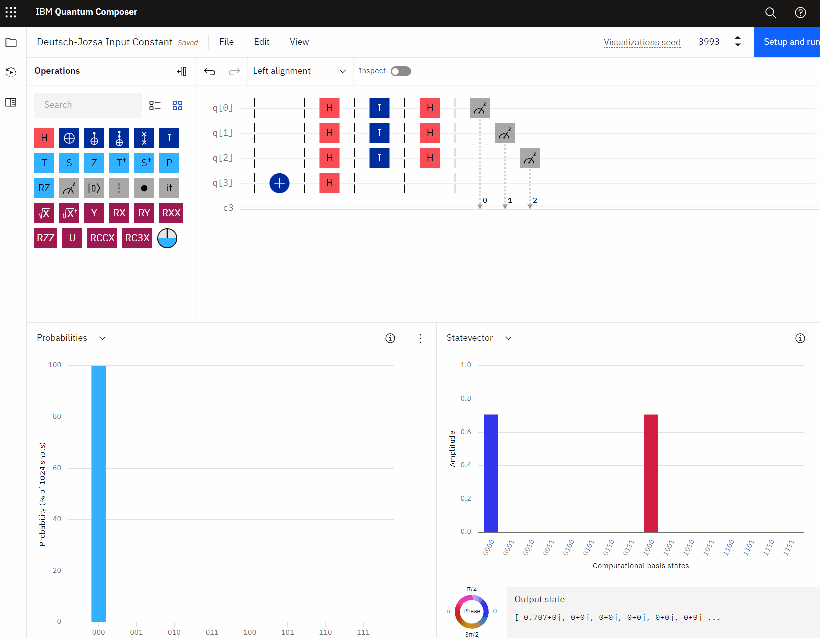
Below is an example of the original algorithm encoded with a constant oracle. Notice, that no matter how the input qubits are modified, the output is always 000 - constant.

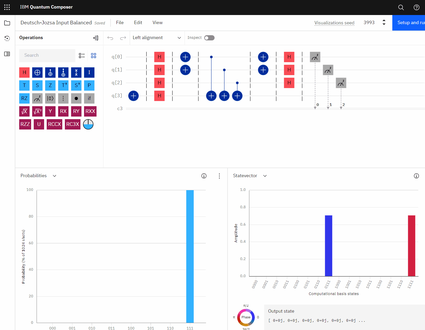
Similarly, here is an example with a balanced oracle. Again, notice how the output remains 111 no matter how the input is changed.

The Enhanced Quantum Program

Let’s see what the enhanced version looks like in the IBM Quantum Composer.

When looking at the screenshots below, note that q3 is the output qubit (the bottom-most digit in the histogram). A value of 1 = constant and 0 = balanced. Essentially, this is the quantum version of the javascript example above for isConstant().

Also notice that as the input qubits are changed, the output changes accordingly, indicating whether the input array is constant (all 0’s or all 1’s) or balanced (a mix of 0’s and 1’s).

Even more impressive, notice how the quantum simulator provides an answer, for the entire array, in just one single execution!

Recall, in the javascript version above, we had to iterate over all values in the array, one at a time, and count up the number of times that we’ve seen a zero or one.

The quantum computer does this simultaneously and instantly returns a result!

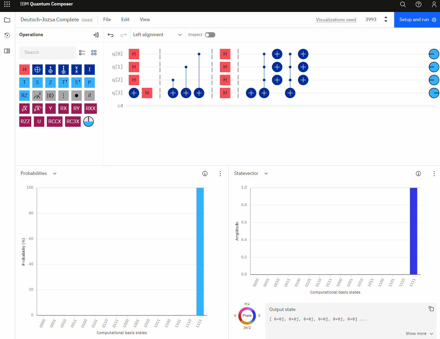
You may have noticed the empty barrier commands in the quantum circuit (vertical dashed lines). This is actually where the oracle would be placed, which encodes the array into controlled NOT gates. The control is the input qubit with a value of 1 while the target is the auxiliary output qubit.

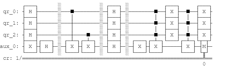
We can actually simplify the circuit by just using X-gates on the input qubits instead, as shown below.

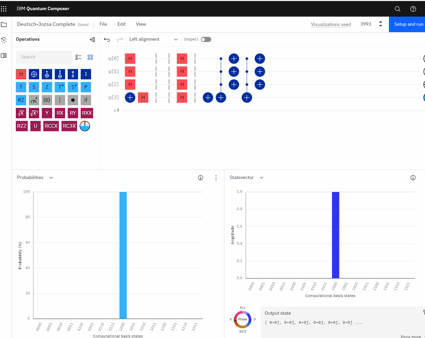
It can be quite interesting to play with the input qubits and see how the output changes, correctly identifying the array as constant or balanced. As X operators are added to the input qubits to flip them to 1, the output changes accordingly, labeling the array as balanced - until all input qubits are either all 1 or all 0, at which point, it flips back to a label of 0 constant.

Building the Circuit in Qiskit

The IBM Quantum Composer is a great way to quickly mock-up a quantum computing circuit to see how it executes. We’ve successfully demonstrated the enhanced algorithm.

Let’s see what the qiskit code would look like. You can enter the code below into a Jupyter Notebook or a .py program.

from qiskit import qiskit, QuantumRegister, ClassicalRegister, QuantumCircuit, Aer
from qiskit.visualization import plot_histogram

qr = QuantumRegister(3, 'qr')
aux = QuantumRegister(1, 'aux')
cr = ClassicalRegister(1, 'cr')
qc = QuantumCircuit(qr, aux, cr)

# Set the output qubit to 1 and place it in superposition.
qc.x(aux)
qc.h(aux)

# Set each input qubit to superposition.
qc.h(qr)
qc.barrier()

# Apply the oracle, encoding input qubits with a value of 1 as a control and the output qubit as the target.
# Example: 101
qc.cx([0, 2], aux)
qc.barrier()

# Bring the qubits out of superposition
qc.h(qr)
qc.h(aux)
qc.barrier()

# Invert the output qubit back to 0.
qc.x(aux)

# Invert the output to 1 if all inputs are 1.
qc.mcx(qr, aux)
qc.x(qr)
qc.mcx(qr, aux)

qc.x(qr)

# Measure the output qubit.
qc.measure(aux, cr)

If we draw the resulting circuit for the input array [1, 0, 1], we can see a diagram perfectly matching the IBM Quantum Composer version.

qc.draw()

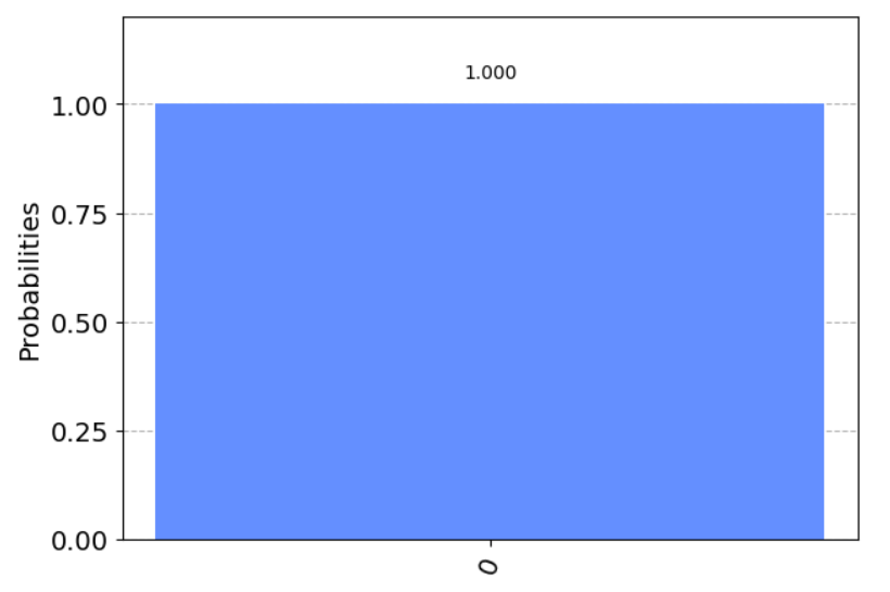
Finally, we can execute the circuit to see the result. This is the same result as we’ve just seen with the IBM Quantum Composer.

backend = Aer.get_backend('aer_simulator')

job = qiskit.execute(qc, backend)
result = job.result()
counts = result.get_counts()
plot_histogram(counts)

The array is balanced.

A Note on the Simulator

The above example measures the output qubit, forcing the resulting output to a single value of 0 - balanced or 1 - constant. We can actually remove the measurement instruction and omit the classical register, using a state-vector simulator to view the result without measuring the output.

backend = Aer.get_backend('statevector_simulator')

job = qiskit.execute(qc, backend)
result = job.result()
counts = result.get_counts()
plot_histogram(counts)

For the state-vector simulator, we’ve removed the classical register from the circuit and also removed the measure instruction. The resulting output now shows all qubits, but retains the correct output qubit value of 0 for balanced and 1 for constant.

One Final Enhancement

As a final touch to our enhanced algorithm, let’s allow the user to pass any input into the circuit. We can do this by adjusting the oracle dynamically to set the controlled-NOT gate on the corresponding qubit accordingly.

def oracle(qr, output, arr):
    qc = QuantumCircuit(qr, aux)

    for i in range(len(arr)):
        if arr[i] == '1':
            qc.cx(qr[i], aux)

    result = qc.to_gate()
    result.name = 'input'

    return result

Our circuit now appears as follows.

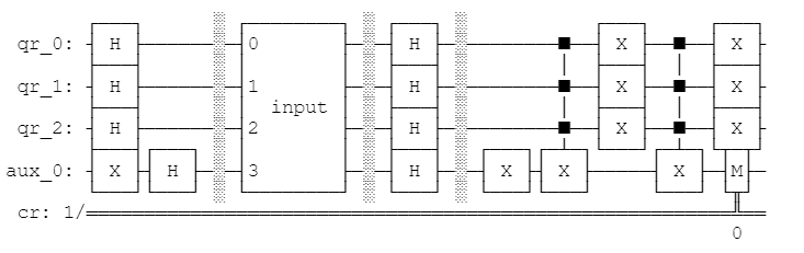
Our “oracle” now consists of an encoding of the input array by flipping the values for the corresponding qubits to 1. This is why the oracle is named “input” - it’s simply an encoding of the input array.

We also no longer use a hard-coded oracle of constant or balanced. Instead, we determine this automatically at execution time.

Wrapping It All Together

Finally, let’s wrap everything up into a tidy method for execution on any input array.

def dj(arr):
    n = len(arr)

    qr = QuantumRegister(n, 'qr')
    aux = QuantumRegister(1, 'aux')
    cr = ClassicalRegister(1, 'cr')
    qc = QuantumCircuit(qr, aux, cr)

    # Set the output qubit to 1 and place it in superposition.
    qc.x(aux)
    qc.h(aux)

    # Set each input qubit to superposition.
    qc.h(qr)
    qc.barrier()

    # Apply the oracle, encoding input qubits with a value of 1 as a control and the output qubit as the target.
    qc.append(oracle(qr, aux, arr), range(len(qr) + 1))
    qc.barrier()

    # Bring the qubits out of superposition
    qc.h(qr)
    qc.h(aux)
    qc.barrier()

    # Invert the output qubit back to 0.
    qc.x(aux)

    # Invert the output to 1 if all inputs are 1.
    qc.mcx(qr, aux)
    qc.x(qr)
    qc.mcx(qr, aux)

    qc.x(qr)

    # Measure the output qubit.
    qc.measure(aux, cr)

    # Execute the circuit.
    backend = Aer.get_backend('aer_simulator')

    job = qiskit.execute(qc, backend)
    result = job.result()
    counts = result.get_counts()

    return counts

We can now execute the Deutsch-Jozsa algorithm on any input array of any length!

counts = dj('100') # 0 balanced
counts = dj('111') # 1 constant
counts = dj('00000') # 1 constant
counts = dj('10110010101100') # 0 balanced

Conclusion

Did you notice in the final example above, we’re passing the entire array of zeroes and ones to the quantum computer to execute in a single call? This one single call outputs constant or balanced.

In order to do the same thing on a classical computer, such as using the isConstant() method that we wrote in javascript earlier, we would need to traverse the array, one index at a time, before we can arrive at an answer.

This, alone, is the difference between (n / 2) + 1 operations on a classical computer versus one single operation on a quantum computer.

It’s almost like magic!

Download @ GitHub

The source code for this project is available on GitHub.

About the Author

This article was written by Kory Becker, software developer and architect, skilled in a range of technologies, including web application development, artificial intelligence, machine learning, and data science.

Sponsor Me